Music.
Regardless of the context in space or time, this simple word can evoke millions of melodies, rythms, artists that have influenced our lives. Music has followed us for our whole lifes, given shape and embelished our best memories.
We want to share our enthusiasm with our visualization project "Evolution of Rock Music" that is based on the widely used dataset "Million songs".
This process book hopefully shed lights into our thought process during the establishment of our visualization, from the choice of the subject to the final touch of the visualization technique used.
For this visualization we focused our energy on Rock Music. Why Rock Music ? First of all, Rock music was a uninanimous choice in terms of music taste in our team so it's only natural to choose the genre that suits us the best. We were really motivated to know more about the subgenres we like the most, and to expand our music knowledge by discovering other styles ! We also want to reach the maximum of audience with our visualization, that is meant to be easy to understand and instructive. Rock with its many subgenres, covers a large scope of the music produced in the western countries for the past 70 years and we believe that everyone knows at least some songs from iconic artists and groups like Elvis Presley, The Beatles and even Michael Jackson. Hopefully we can provide a good explanation of rock music through our visualization and hopefully even surprise the rock pundits !
Throughout the course of Data Visualization this semester, we had the chance to have a look at all sort of visualizations. One graph that suits very well our project of showing the evolution of Rock music in time is the stream graph. It's a time based graph comprising different colors that represent our various subgenres. This visualization gives an a lot of information while remaining fairly simple to read.
This is an example of streamgraph that caught our eye. It represents the evolution of music genre at the Montreux Jazz Festival. Each color represents a genre with the possibility to have additional information by hovering over the different colored areas. See original work
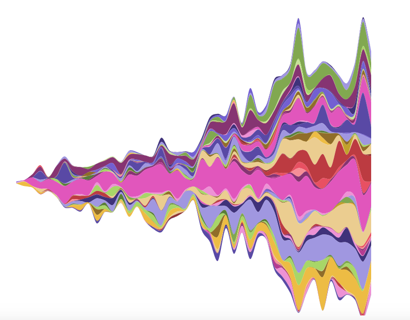
Courtesy of Maximilien Cuony and Kirell Benzi, taken from http://www.kirellbenzi.com/.
For the structure of our visualization and especially the story telling we wanted to combine them in the same page. This was decided after looking at this interactive visualization that showed the number of attacks by drone in Pakistan. We think that the user would be more inclined to be interested and focused in our visualization if we guide him/her with a demo-like story telling.
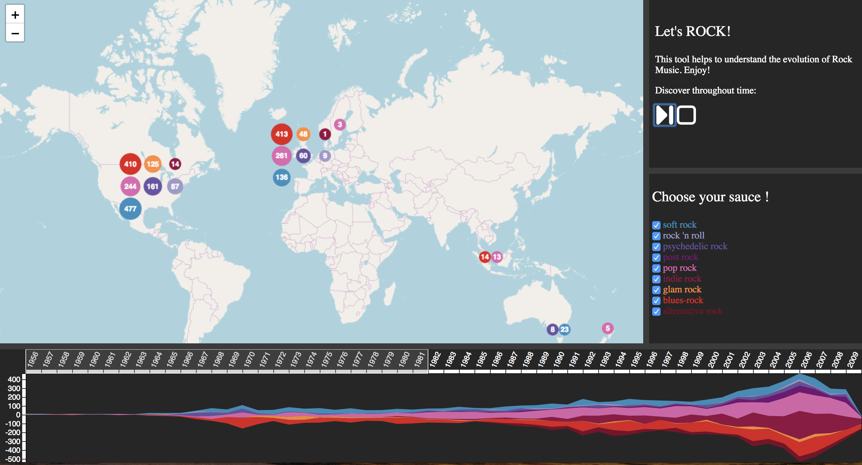
The main goal of our visualization is to show the evolution of Rock Music in time and space. With our structure, we can assess both variables via our streamgraph with the brusher associated, and the map. We can see the markers appear more and more in Europe for example as we move the brush in time. More specifically, we added 9 subgenres of Rock so the user can have an understanding of the different style of Rock first of all, but also their popularity and their evolution in time. Finally, each icon representing one song carry the information of the name of the song, the artist name, the genre and the hotness (measured in by The Echo Nest following their criterion). It's a more detailed information for the users who want to discover new musics, new genres from various countries. There are many ways to use our visualization, each type of user can find its own preference. Our story telling focus on different eras of Rock music, by highlighting the main subgenres and the notable artists or groups.
The Million Song Dataset with its abundant and detailed features for each song is such an incredible source for data treatment. In our case, we had to do a fair bit of data analysis to understand its nature in order to grasp the potential for a visualization. The full dataset is available in the cluster of the EPFL so we had to write a script (GetData.py) to retrieve all the important features that would have meaning for our visualization. For example, features like the BPM, segments_loudness_start that are more focused toward music analysis were left off to save some computation time and memory. (The whole Million Song Dataset is 280 GB in size). Because our visualization is based on the map and on a streamgraph, the location of the artist and the year of the song release is mandatory. We used Python and Spark (PySpark) to read the files in h5py, filter them by years and locations and used hd5f_getters.py, a file provided by LabROSA who designed the dataset with The Echo Nest to get the different features of interest for each song:
   - Year
   - Artist latitude
   - Artist longitude
   - Artist hotness
   - Artist name
   - Artist id
   - Artist terms (First 10 genre associated to the artist)
   - Title of the song
   - Song hotness
If one does not have access to the EPFL cluster, the full dataset and a subset can be downloaded here
Because there have been so many genres of rock since the 50s, we decided to focus our attention toward those following ones:
   - pop rock
   - blues-rock
   - indie rock
   - post rock
   - psychedelic rock
   - rock 'n roll
   - alternative rock
   - glam rock
   - soft rock
They cover all eras of rock pretty well and are the most popular and well known subgenre of rock. A main giveaway about the treatment of the data is that there are a lot of missing features in the dataset which make the filtering very selective.
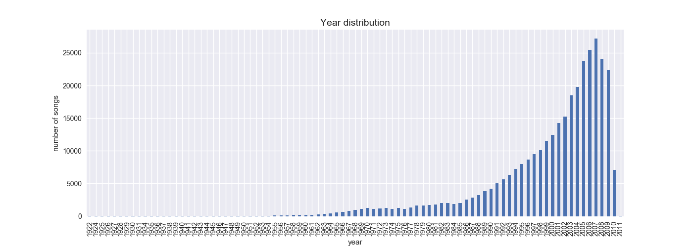
For exploratory visualization, we used python to plot some graphs to gain more insights on the dataset. The first key information to follow is the distribution of songs by time. This gives a good indicator of the number of songs in the dataset for each year. It shows that most of the songs in the dataset are quite recent (last decade and a half). Even so, still a great number of songs are present in the dataset ranging from the 50s to the early 2000s.
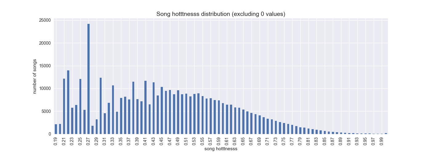
There was also a deep interest in the hotness of the song at the begining of the project, which led us to visualize its ditribution for a range of hotness.
We also used a python package called folium to buid a map to have a quick overview of the distribution of songs in the world, to verify that the artist locations are coherent. (For example Vanessa Paradis in France).
Our visualization is based on a Leaflet map coupled with a svg streamgraph.
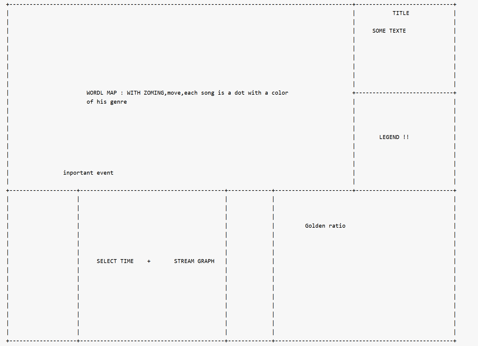
This was the first sketch that was made when we came up with the idea. Overall, if we compare it to the final visualization, it shows that we stayed in the same line of work, at least in terms of strucutre.
Initially, we wanted to show the evolution of all types of music thoughout the past century in the world in order to understand the different eras of music by country. The idea was to highlight the evolution of one or two features of a song (e.g. hotness,danceability) by country in time. As a visualization we had the intention to use a 2D scatter plot with a slider to navigate in time. See example
We tought that the subject was too wide and not specific enough to convey a clear enough message to the viewer. The scatter plot is a bit simplistic as a visualization method and also difficult to interpret so we decided to have more meaningful approach with the map and the streamgraph.
As a starter, the aim was to divide the window as shown in the sketch, hence allocating most of the areas to the map and the streamgraph. Each area of the visualization should be stretchable with the proper resizing.
This first visualization was done with 10 points which explains the awkward shape of the stream graph.
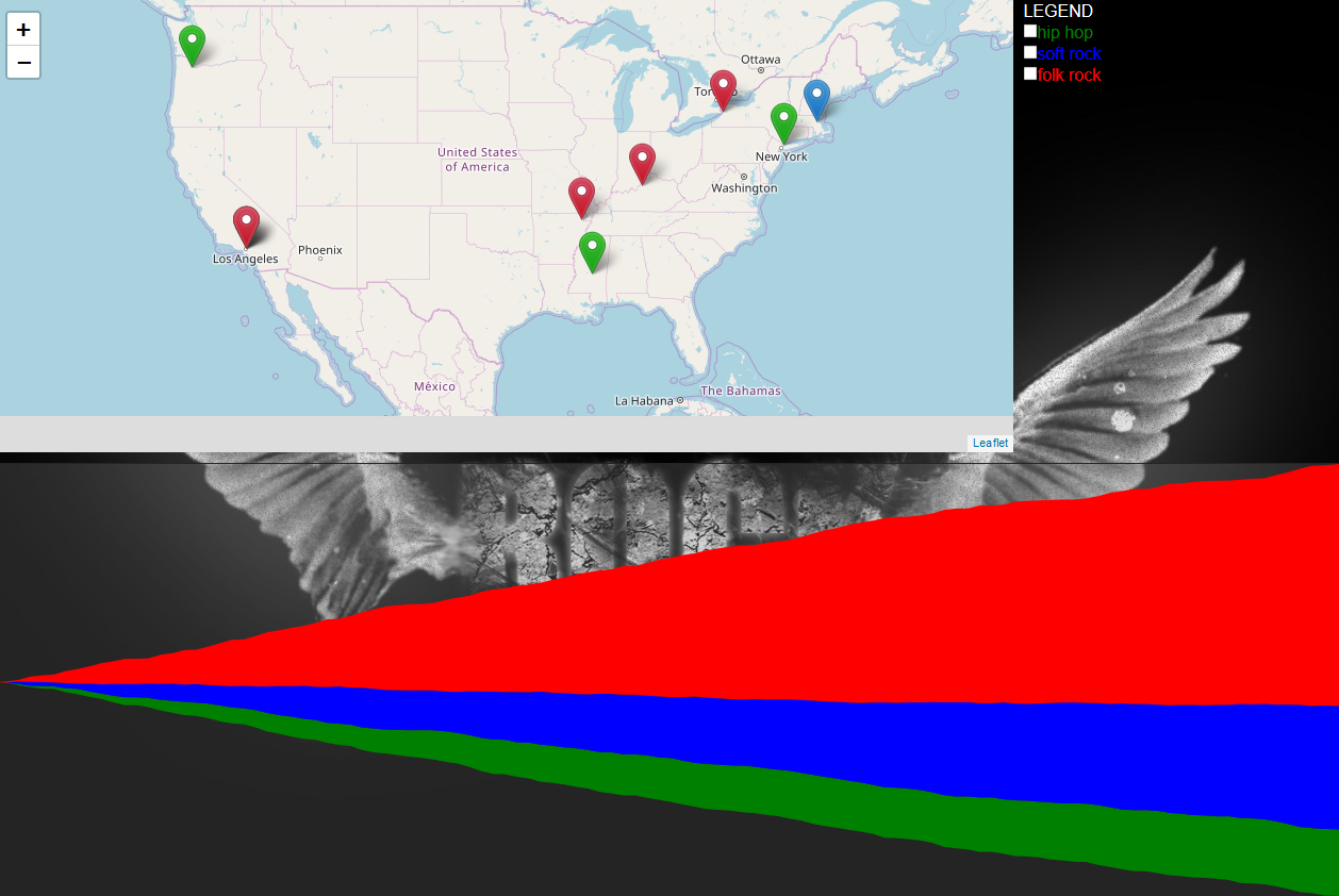
Having data with geographical location and realease years of songs pushed us towards using a map and a sreamgraph. The streamgraph shoulh give a quick overview of the split of the styles throughout years and the map should split the data geographically. Morevover, we want two graphs to be connected and originally we wanted to use years on x-axis of the streamgraph to filter the data shown on the map, so to show only songs released during selected time range. Another filter that we though of were styles. We wanted to be able to see the progression of only one style on the map, so we added a simple filter with checkboxes in the 'legend' part of the screen. This filter allows to check/unckeck any style available, so we can see any number of available styles on the map. The result of this version can be seen on this screenshot
The were a few issues we've encountered. First of all, the markers on the map. There were too many overlapping markers in the same locations and they were too big. Secondly, our time brush was on the streamgraph, which made it impossible to make the streamgraph interactive directly. So, we have decided to move the time range selector on the top of the graph, making it a separate selector over the x-axis of the streamgraph.
Another issue we've noticed was the way the time range was selected. In our dataset we have only years, but with the brush selector we could stop anywhere on the timeline. So we've decided to split the timeline clearly by years and make the selector round to the closest year.
For the map we have decided to use some clustering of the data points. At every zoom level we can see a few clusters of data, represented by bubbles. In order to see the number of points in the cluster and song styles, we made the cluster bubble outline colored with styles (like in a pie chart), with the number of points in the middle of the bubble.
This version can be viewed on this screenshot together with the experimental background :)
By observing the results of version 2, we have noticed that it was hard to observe the progression through time, as the cluster bubbles were of the same size and grasping the numbers of all to see which one is bigger was sometimes difficult, especially when going through time automatically, with the help of the button in the upper right part of the screen. Another issue with cluster bubbles was their segmentation in styles: since the coloring was proportional to all styles available in that cluster, it wasn't comparable to other clusters. Thus, it was impossible to see from first glance which style was dominant in selected time range and where.
Another option we've tried out was changing the streamgraph. We wanted to be able to show different styles on it, so we made style filter change the graph too (together with the map). However, since we wanted to filter the map by also clicking on the style on the streamgraph (which would also tick or untick the corresponding boxes in the filter), this new option didn't make sense, so we have decided to give it up and just keep the filtering of the map available through the ticking of the box or selecting on the streamgraph.
Our solution to the map was the following: we decided to keep the clusters, however slightly different. Why so? Because of how data points were spread out on the map. The problem is that most of the points actually map to the same locations, like centers of big cities. So, in the end, a lot of points map to the same locations and overlap, so it becomes impossible to see which styles are represented in those locations. We have tried to overcome this issue by introducing some randomness for those locations, but this was distorting out data and eventially it wasn't what we wanted. The fact that the data points were overlapping a lot was also the reason why we've decided to give up on dot distribution map. Even with introduced randomness, the following was the best result we have obtained and as it can be seen from the screenshot, it is difficult to separate points and see which style (which color) has the most points.
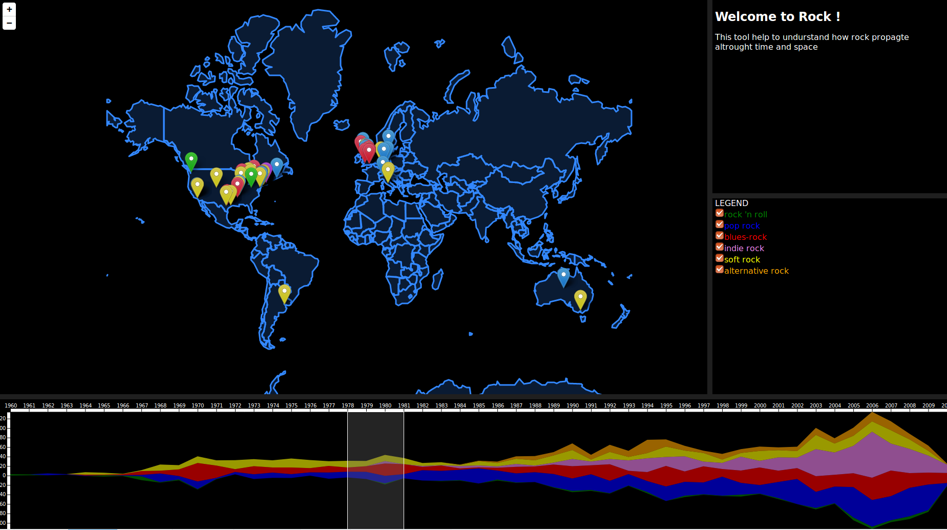
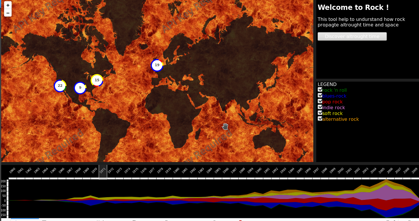
Here's how we changed the clusters. First of all, we decided to separate each style, so now every cluster is not one bubble, but as many bubbles as there are styles in this cluster. Secondly, the size of each bubble is proportional to the number of data points it represents, so bigger clusters are bigger in size. Like this dominant styles can be instantly seen on the map. Clusterin itself works as before: as you zoom in, the clusters are reformed, allowing to group data points more locally and so see more details on every zoom level in. Below is the screenshot of the map at this stage.

Here's a few things we have come up after discussing out version 3. We have decided to make the time range selector easier: since in order to select one year, one need to find and drag the brush from both sides, we have decided to make that available with on click on the year. Another thing that we finally decided to work on is the styling and shaping of the web page (since some of our elements and text we going out from the page). Another thing we tried to do was to set max zoom for the map and limit it, so it won't be possible to scroll too far on it, but we still need to adjust a few things there. In terms of automatic time view, we decided that we need at least play, stop and pause buttons, for user to have some control over the timeplay.
Here's our version at this point:
We decided that additional options for playing such as speed selector would be a nice thing to have, too.
The problem we have now is how to make everything look coherent and integrated together. We decided that we need to change the color of the map background, remove y-axis from the streamgraph, reposition some elements on the page and show some information on hover for the streamgraph and map (on the bubbles).
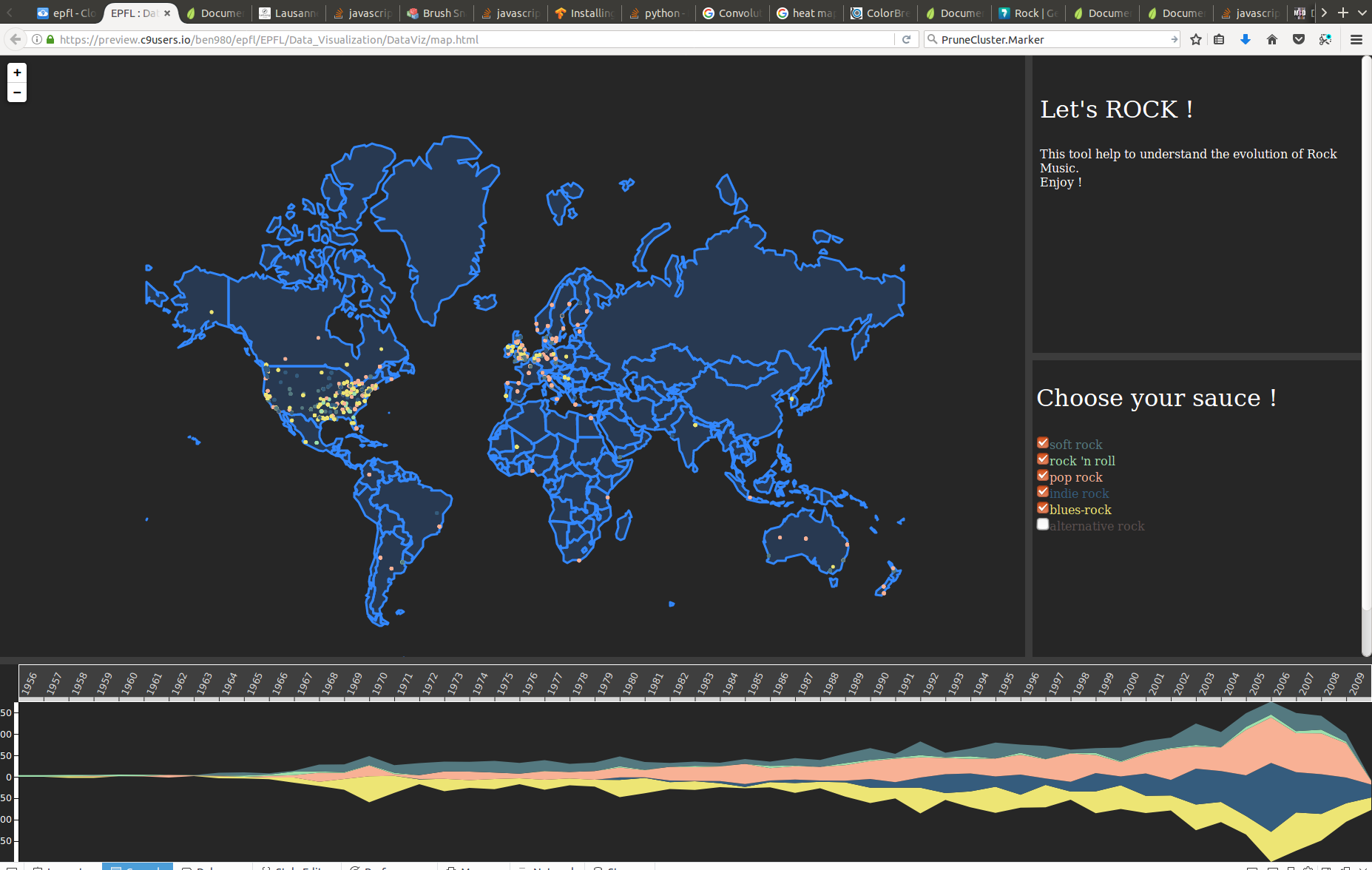
Here is our final version.

So what are the different features of our visualization. First of all we removed the legend area and moved it inside the map. We feel it makes the experience of the user smoother and the addition of the colored circles next to the text instead of the check boxes makes the genres blend in the dark background better. There are some buttons on the left-bottom side of the screen that can be used to control the demo of the story telling. During this demo, the brusher under the stream graph moves automatically, starting from the first year (1956) with a story about Little Richard and Rock and Roll. The cluster on the map shows the number of songs in the proximate areas. The more you zoom the more clusters you see. At the max zoom level, the icons containing the information of the song can be seen. Finally we added some information when hovering over the streamgraph.
To improve our our visualization we could have added the link to the corresponding song via a music platform. Some additional interactions with the streamgraph could have been added. Also it would be a good idea to add more transition after each events so the navigation can be smoother. The demo also needs to be more interactive. It should maybe zoom on an icon, display some texts giving a little explanation. (Similar to the story telling in the screencast)
There are actually so many possibilities with our topic and our visualization.
Paul
- Preparation : My teammates were ready each tuesday to debate for hours about the projects
- Contribution : Yes we separated the different tasks based on our skills
- Respect for other's ideas : Yes the art of criticizing with respect
- Flexibility : Yes flexible enough
Olga
- Preparation : Yes, what Paul said :)
- Contribution : Everyone had great ideas, which helped to move the project quickly
- Respect for other's ideas : Yes, everyone would listen to the other's opinion
- Flexibility : Yes
Benjamin :
- Preparation : Yes !
- Contribution : Everybody has a slow start a first, but at the end everyone work efficienly
- Respect for other's ideas : Yep, everybody takes into account what the other say
- Flexibility : Yes , but we never have true disagreements, but some difficulty sometime to understand each other due to the english/french language.