Singular value decomposition is an extension of eigenvector decomposition of a matrix.
For the square matrix
Theorem: All eigenvalues of a symmetrical matrix are real.
Proof: Let
$A$ be a real symmetrical matrix and$Av=\lambda v$ . We want to show the eigenvalue$\lambda$ is real. Let$v^{\star}$ be conjugate transpose of$v$ .$v^{\star}Av=\lambda v^{\star}v,(1)$ . If$Av=\lambda v$ ,thus$(Av)^{\star}=(\lambda v)^{\star}$ , i.e.$v^{\star}A=\bar{\lambda}v^{\star}$ . We can infer that$v^{\star}Av=\bar{\lambda}v^{\star}v,(2)$ .By comparing the equation (1) and (2), we can obtain that$\lambda=\bar{\lambda}$ where$\bar{\lambda}$ is the conjugate of$\lambda$ .
Theorem: Every symmetrical matrix can be diagonalized.
See more at http://mathworld.wolfram.com/MatrixDiagonalization.html.
When the matrix is rectangle i.e. the number of columns and the number of rows are not equal, what is the counterpart of eigenvalues and eigenvectors?
Another question is if every matrix
They are from the square matrices
Theorem: The matrix
$A$ and$B$ has the same eigenvalues except zeroes.Proof: We know that
$A=M_{m\times n}^TM_{m\times n}$ and$B=M_{m\times n}M_{m\times n}^T$ . Let$Av=\lambda v$ i.e.$M_{m\times n}^TM_{m\times n} v=\lambda v$ , which can be rewritten as$M_{m\times n}^T(M_{m\times n} v)=\lambda v,(1)$ , where$v\in\mathbb{R}^n$ . We multiply the matrix$M_{m\times n}$ in the left of both sides of equation (1), then we obtain$M_{m\times n}M_{m\times n}^T(M_{m\times n} v)=M_{m\times n}(\lambda v)=\lambda(M_{m\times n} v)$ such that$B(M_{m\times n}v)=\lambda M_{m\times n}v$ .
Another observation of
Theorem: The matrix
$A$ and$B$ are non-negative definite, i.e.$\left<v,Av\right>\geq 0, \forall v\in\mathbb{R}^n$ and$\left<u,Bu\right>\geq 0, \forall u\in\mathbb{R}^m$ .Proof: It is
$\left<v,Av\right>=\left<v,M_{m\times n}^TM_{m\times n}v\right>=(Mv)^T(Mv)=|Mv|_2^2\geq 0$ as well as$B$ .
We can infer that the eigenvalues of matrix
The eigenvalues of
It is known that
Theorem:
$M_{m\times n}=U_{m\times m}\Sigma_{m\times n} V_{n\times n}^T$ , where
$U_{m\times m}$ is an$m \times m$ orthogonal matrix;$\Sigma_{m\times n}$ is a diagonal$m \times n$ matrix with non-negative real numbers on the diagonal,$V_{n\times n}^T$ is the transpose of an$n \times n$ orthogonal matrix.
| SVD |
|---|
 |
See more at http://mathworld.wolfram.com/SingularValueDecomposition.html.
- http://www-users.math.umn.edu/~lerman/math5467/svd.pdf
- http://www.nytimes.com/2008/11/23/magazine/23Netflix-t.html
- https://zhuanlan.zhihu.com/p/36546367
- http://www.cnblogs.com/LeftNotEasy/archive/2011/01/19/svd-and-applications.html
- Singular value decomposition
- http://www.cnblogs.com/endlesscoding/p/10033527.html
- http://www.flickering.cn/%E6%95%B0%E5%AD%A6%E4%B9%8B%E7%BE%8E/2015/01/%E5%A5%87%E5%BC%82%E5%80%BC%E5%88%86%E8%A7%A3%EF%BC%88we-recommend-a-singular-value-decomposition%EF%BC%89/
- https://www.wikiwand.com/en/Singular_value
It is to maximize the variance of the data projected to some line, which means compress the information to some line as much as possible.
Let
$$Y=\arg\max{Y} , var(Y)=w^{T}\Sigma w, \text{s.t.} w^T w={|w|}_2^2=1 .$$
It is a constrained optimization problem.
| Gaussian Scatter PCA |
|---|
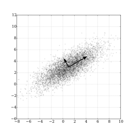 |
- Principal Component Analysis Explained Visually.
- https://www.zhihu.com/question/38319536
- Principal component analysis
- https://www.wikiwand.com/en/Principal_component_analysis
- https://onlinecourses.science.psu.edu/stat505/node/49/
In linear regression, we assume that
- https://www.jianshu.com/p/d090721cf501
- https://www.wikiwand.com/en/Principal_component_regression
- http://faculty.bscb.cornell.edu/~hooker/FDA2008/Lecture13_handout.pdf
- https://learnche.org/pid/latent-variable-modelling/principal-components-regression
PCA can extend to generalized principal component analysis(GPCA), kernel PCA, functional PCA. The generalized SVD also proposed by Professor Zhang Zhi-Hua. SVD as an matrix composition method is natural to process the tabular data. And the singular values or eigenvalues can be regarded as the importance measure of features or factors. And it used to dimension reduction.
- http://people.eecs.berkeley.edu/~yima/
- http://www.cis.jhu.edu/~rvidal/publications/cvpr03-gpca-final.pdf
- http://www.vision.jhu.edu/gpca.htm
- http://www.psych.mcgill.ca/misc/fda/files/CRM-FPCA.pdf
- https://www.wikiwand.com/en/Kernel_principal_component_analysis
- https://arxiv.org/pdf/1510.08532.pdf
- http://www.math.pku.edu.cn/teachers/zhzhang/