Let's start simple, highlighting some basic tools that we will need later: chiefly, tools from the broom package.
Hadley (Wickham, 2014) puts this well:
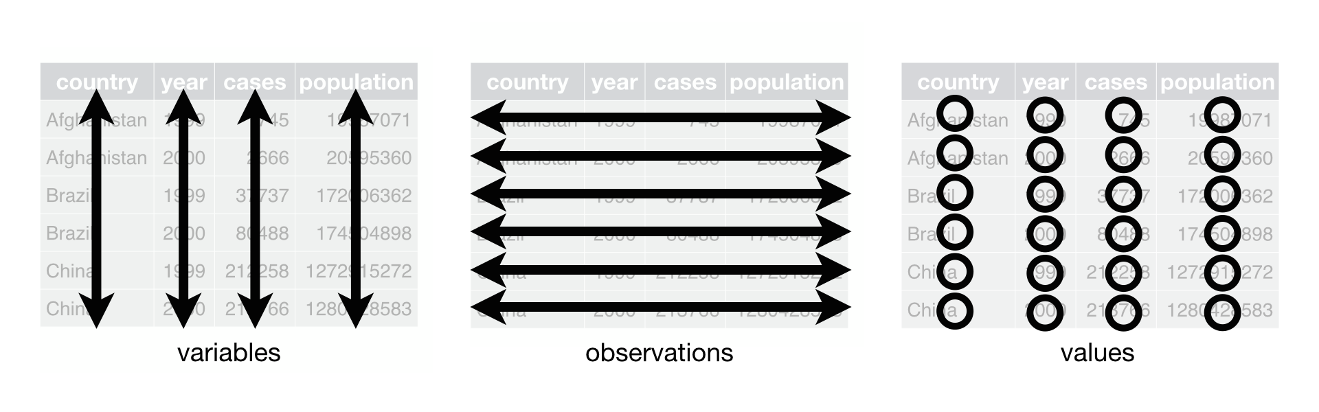
"tidy datasets provide a standardised way to link the structure of a dataset (its physical layout) with its semantics (its meaning)"
Appearance layout of tidy data:
- Each variable is represented by a single column
- each observation has its own row
- each value has its own cell
More info: https://github.com/egouldo/VicBioCon17_data_wrangling/blob/master/modules/06_tidy_data.md
Regressions are messy in R...
library(magrittr)
lm_car <- lm(mpg ~ wt + qsec, data = mtcars)
summary(lm_car) # messy output
##
## Call:
## lm(formula = mpg ~ wt + qsec, data = mtcars)
##
## Residuals:
## Min 1Q Median 3Q Max
## -4.3962 -2.1431 -0.2129 1.4915 5.7486
##
## Coefficients:
## Estimate Std. Error t value Pr(>|t|)
## (Intercept) 19.7462 5.2521 3.760 0.000765 ***
## wt -5.0480 0.4840 -10.430 2.52e-11 ***
## qsec 0.9292 0.2650 3.506 0.001500 **
## ---
## Signif. codes: 0 '***' 0.001 '**' 0.01 '*' 0.05 '.' 0.1 ' ' 1
##
## Residual standard error: 2.596 on 29 degrees of freedom
## Multiple R-squared: 0.8264, Adjusted R-squared: 0.8144
## F-statistic: 69.03 on 2 and 29 DF, p-value: 9.395e-12
- Extracting coefficients takes multiple steps
data.frame(coef(summary(lm_car))) - Information is stored in rownames: combining models requires wrangling
- Column names are annoying: must access with
$“Pr(>|t|)”, and is converted toPr...t.. - Information computed in the print method is not stored, e.g. F-stat and p-values
# Enter broom:
library(broom)
Broom generates tidy model summaries, turning statistical models into tidy data-frames.
-
broom::tidymodel component-level statistics: coefficient estimates, SE, etc. -
broom::augmentobservation-level, fitted values, residuals etc. -
broom::glance- model-level statistics: e.g.${R}^{2}$ , AIC, deviance etc.
lm_car %>% broom::tidy() # one observation per model term## term estimate std.error statistic p.value
## 1 (Intercept) 19.746223 5.2520617 3.759709 7.650466e-04
## 2 wt -5.047982 0.4839974 -10.429771 2.518948e-11
## 3 qsec 0.929198 0.2650173 3.506179 1.499883e-03
lm_car %>% broom::augment() # one observation per observation in the original data, new columns preceded with "."## .rownames mpg wt qsec .fitted .se.fit .resid
## 1 Mazda RX4 21.0 2.620 16.46 21.815109 0.6832424 -0.81510855
## 2 Mazda RX4 Wag 21.0 2.875 17.02 21.048224 0.5468271 -0.04822401
## 3 Datsun 710 22.8 2.320 18.61 25.327279 0.6397681 -2.52727880
## 4 Hornet 4 Drive 21.4 3.215 19.44 21.580569 0.6231436 -0.18056924
## 5 Hornet Sportabout 18.7 3.440 17.02 18.196114 0.5120709 0.50388581
## 6 Valiant 18.1 3.460 20.22 21.068588 0.8032106 -2.96858808
## 7 Duster 360 14.3 3.570 15.84 16.443423 0.7010125 -2.14342291
## 8 Merc 240D 24.4 3.190 20.00 22.227120 0.7302126 2.17288034
## 9 Merc 230 22.8 3.150 22.90 25.123713 1.4101406 -2.32371308
## 10 Merc 280 19.2 3.440 18.30 19.385488 0.4909773 -0.18548760
## 11 Merc 280C 17.8 3.440 18.90 19.943006 0.5571043 -2.14300639
## 12 Merc 450SE 16.4 4.070 17.40 15.368981 0.6147893 1.03101923
## 13 Merc 450SL 17.3 3.730 17.60 17.271134 0.5204289 0.02886576
## 14 Merc 450SLC 15.2 3.780 18.00 17.390414 0.5387353 -2.19041433
## 15 Cadillac Fleetwood 10.4 5.250 17.98 9.951297 1.0916727 0.44870314
## 16 Lincoln Continental 10.4 5.424 17.82 8.924276 1.1612916 1.47572368
## 17 Chrysler Imperial 14.7 5.345 17.42 8.951388 1.1149850 5.74861230
## 18 Fiat 128 32.4 2.200 19.47 26.732147 0.7508141 5.66785310
## 19 Honda Civic 30.4 1.615 18.52 28.802478 0.8918780 1.59752172
## 20 Toyota Corolla 33.9 1.835 19.90 28.974215 0.9091942 4.92578455
## 21 Toyota Corona 21.5 2.465 20.01 25.896199 0.7735519 -4.39619858
## 22 Dodge Challenger 15.5 3.520 16.87 17.652896 0.5348830 -2.15289593
## 23 AMC Javelin 15.2 3.435 17.30 18.481530 0.4873703 -3.28152953
## 24 Camaro Z28 13.3 3.840 15.41 14.680913 0.8069223 -1.38091265
## 25 Pontiac Firebird 19.2 3.845 17.05 16.179557 0.5703305 3.02044258
## 26 Fiat X1-9 27.3 1.935 18.90 27.540219 0.7829311 -0.24021927
## 27 Porsche 914-2 26.0 2.140 16.70 24.461147 0.7941163 1.53885259
## 28 Lotus Europa 30.4 1.513 16.90 27.812072 1.0132627 2.58792829
## 29 Ford Pantera L 15.8 3.170 14.50 17.217490 1.0029250 -1.41749041
## 30 Ferrari Dino 19.7 2.770 15.50 20.165881 0.8318811 -0.46588119
## 31 Maserati Bora 15.0 3.570 14.60 15.291217 0.9642049 -0.29121742
## 32 Volvo 142E 21.4 2.780 18.60 22.995915 0.5294628 -1.59591510
## .hat .sigma .cooksd .std.resid
## 1 0.06925986 2.637300 2.627038e-03 -0.32543724
## 2 0.04436414 2.642112 5.587076e-06 -0.01900129
## 3 0.06072636 2.595763 2.174253e-02 -1.00443793
## 4 0.05761138 2.641895 1.046036e-04 -0.07164647
## 5 0.03890382 2.640343 5.288512e-04 0.19797699
## 6 0.09571739 2.575422 5.101445e-02 -1.20244126
## 7 0.07290940 2.608421 1.927373e-02 -0.85745788
## 8 0.07910987 2.607247 2.178198e-02 0.87216352
## 9 0.29502367 2.589845 1.585198e-01 -1.06600994
## 10 0.03576473 2.641888 6.545298e-05 -0.07275945
## 11 0.04604739 2.609389 1.149236e-02 -0.84513499
## 12 0.05607697 2.634506 3.308687e-03 0.40875633
## 13 0.04018415 2.642123 1.797445e-06 0.01134893
## 14 0.04306089 2.608022 1.115778e-02 -0.86248219
## 15 0.17681412 2.640475 2.598066e-03 0.19049175
## 16 0.20008504 2.623664 3.367812e-02 0.63554917
## 17 0.18444635 2.352379 4.532124e-01 2.45190009
## 18 0.08363669 2.393496 1.582375e-01 2.28060859
## 19 0.11801654 2.622499 1.914813e-02 0.65521310
## 20 0.12264373 2.448094 1.911855e-01 2.02559882
## 21 0.08877914 2.494666 1.021948e-01 -1.77390963
## 22 0.04244725 2.609209 1.061160e-02 -0.84743754
## 23 0.03524115 2.565582 2.016397e-02 -1.28686488
## 24 0.09660408 2.627824 1.116304e-02 -0.55961992
## 25 0.04825977 2.576528 2.403811e-02 1.19255217
## 26 0.09094506 2.641700 3.140692e-04 -0.09704626
## 27 0.09356216 2.624412 1.333611e-02 0.62257836
## 28 0.15232675 2.588179 7.021574e-02 1.08268973
## 29 0.14923442 2.626118 2.048803e-02 -0.59194477
## 30 0.10267260 2.640493 1.368718e-03 -0.18943740
## 31 0.13793379 2.641464 7.784575e-04 -0.12081283
## 32 0.04159134 2.624106 5.703374e-03 -0.62791439
lm_car %>% broom::glance() # one observation per model## r.squared adj.r.squared sigma statistic p.value df logLik
## 1 0.8264161 0.8144448 2.596175 69.03311 9.394765e-12 3 -74.36025
## AIC BIC deviance df.residual
## 1 156.7205 162.5834 195.4636 29
Don't know what a pipe (%>%) is? Click here: https://github.com/egouldo/VicBioCon17_data_wrangling/blob/master/modules/05_dplyr-walkthrough.md#writing-sentences-joining-verbs-with-pipes-
- The data manipulation and reshaping is done for you, by
broom. You can focus on understanding your model and your data, rather than on writing code. - Tidy data works with tidy tools: we can easily visualise broom's output with
ggplot, e.g. plotting the model in dataspace, generate coefficient plots, survival curves, etc. - Working with MANY models: tidy model outputs can be easily combined, and compared.
- Exploring the space of all possible models and their relative merits: E.g. for a given model family, you can explore different forms, for example, for a linear model we could generate all models with main effects.
- Varying model settings: e.g. systematically alter the tuning parameters to observe the result.
- Fitting the same model to different datasets: cross-validation, bootstrapping, simulating data, sensitivity analyses, etc.
- Finding global optima - e.g. when model fitting might not converge to global optimum, you can have a collection of models generated from multiple random starts.
- Fitting many simple models ot smaller sub-groups of your data rather than a single complex model to the whole dataset
We can distill the above tasks into two primary workflows:
- When you have a single model that you want to repeatedly fit to different sub-sets of the larger data set.
- When you have a selection of different models you want to fit to the same piece of data repeatedly.
You could solve this computationally by fitting many models using for-loops. Or, when fitting fewer models, you can store your models and their resultant outputs as objects in your global environment.
- Loops: slow, cumbersome to write
- Intermediate objects: clutter up your global environment, must keep mental-track of each object
- For either method, you still need to extract the desired model outputs from each fitted model, wrangle them, combine them, perhaps wrangle some more, before you can analyse and/or visualise your many models simultaneously.
But there are a suite of tools out there that get the job done more efficiently (both in terms of computational efficiency, and in terms of the actual code that you write)!
What do we need? (getting around the loop / many objects conundrum)
- dplyr: create new columns / variables, amend existing ones
- tidyr: nested data with list-columns
- purrr: map functions, map nested dataframes to the modeling function or to broom function
library(dplyr) # data manipulation##
## Attaching package: 'dplyr'
## The following objects are masked from 'package:stats':
##
##     filter, lag
## The following objects are masked from 'package:base':
##
##     intersect, setdiff, setequal, union
library(tidyr) # For reshaping dataframes, specifically nesting##
## Attaching package: 'tidyr'
## The following object is masked from 'package:magrittr':
##
##     extract
library(purrr) # For applying functions to nested dataframes##
## Attaching package: 'purrr'
## The following objects are masked from 'package:dplyr':
##
##     contains, order_by
## The following object is masked from 'package:magrittr':
##
##     set_names
library(ggplot2) # good lookin' plots
spp_mods <- feather::read_feather("./data/grasslands_data")

spp_mods
## # A tibble: 3,874 × 24
## transect_number quadrat species percent_cover origin
## <fctr> <fctr> <fctr> <dbl> <chr>
## 1 1 4 acaena echinata 1.0 N
## 2 1 9 acaena echinata 5.0 N
## 3 2 7 acaena echinata 2.0 N
## 4 2 9 acaena echinata 0.5 N
## 5 5 2 acaena echinata 0.5 N
## 6 5 4 acaena echinata 0.5 N
## 7 7 4 acaena echinata 1.0 N
## 8 11 3 acaena echinata 0.5 N
## 9 11 8 acaena echinata 2.0 N
## 10 12 4 acaena echinata 2.0 N
## # ... with 3,864 more rows, and 19 more variables: growth_form <chr>,
## # type <fctr>, size <dbl>, date <date>, orientation <chr>,
## # assistant <chr>, management <fctr>, burn_season <fctr>,
## # years_since <dbl>, biomass_reduction_year <dbl>,
## # management_unit <fctr>, BG_pc <dbl>, E_pc <dbl>, NF_pc <dbl>,
## # NG_pc <dbl>, BG_diversity <dbl>, E_diversity <dbl>,
## # NF_diversity <dbl>, NG_diversity <dbl>
spp_mods %>%
        ggplot(aes(y = percent_cover, x = BG_pc, colour = type)) +
        geom_point() + facet_grid(~ type)
spp_mods %>%
        ggplot(aes(y = percent_cover, x = E_pc, colour = type)) +
        geom_point() + facet_grid(~ type)
spp_mods %>%ggplot(aes(y = percent_cover, x = E_diversity, colour = type)) +
        geom_point() + facet_grid(~ type)
spp_mods <-
        spp_mods %>%
        group_by(species, type) %>%
        nest()
spp_mods
## # A tibble: 94 × 3
## species type data
## <fctr> <fctr> <list>
## 1 acaena echinata NF <tibble [35 × 22]>
## 2 agrostis capillaris E <tibble [2 × 22]>
## 3 aira caryophyllea E <tibble [214 × 22]>
## 4 anagallis arvensis E <tibble [8 × 22]>
## 5 anthoxanthum odoratum E <tibble [29 × 22]>
## 6 arctotheca calendula E <tibble [26 × 22]>
## 7 arthropodium strictum NG <tibble [14 × 22]>
## 8 asperula conferta NF <tibble [37 × 22]>
## 9 austrostipa spp. NG <tibble [143 × 22]>
## 10 avena fatua / barbata E <tibble [104 × 22]>
## # ... with 84 more rows
List-columns are great because they keep all related objects together (i.e. in a row). We do not have to keep them manually in sync - the dataframe structure does this for us.
species_model <- function(dataframe){
        lm(percent_cover ~ BG_pc + E_pc + E_diversity + management, data = dataframe)
}

spp_mods <-
        spp_mods %>%
        mutate(model = purrr::map(data, species_model))
spp_mods
## # A tibble: 94 × 4
## species type data model
## <fctr> <fctr> <list> <list>
## 1 acaena echinata NF <tibble [35 × 22]> <S3: lm>
## 2 agrostis capillaris E <tibble [2 × 22]> <S3: lm>
## 3 aira caryophyllea E <tibble [214 × 22]> <S3: lm>
## 4 anagallis arvensis E <tibble [8 × 22]> <S3: lm>
## 5 anthoxanthum odoratum E <tibble [29 × 22]> <S3: lm>
## 6 arctotheca calendula E <tibble [26 × 22]> <S3: lm>
## 7 arthropodium strictum NG <tibble [14 × 22]> <S3: lm>
## 8 asperula conferta NF <tibble [37 × 22]> <S3: lm>
## 9 austrostipa spp. NG <tibble [143 × 22]> <S3: lm>
## 10 avena fatua / barbata E <tibble [104 × 22]> <S3: lm>
## # ... with 84 more rows
spp_mods <-
        spp_mods %>%
        dplyr::mutate(coefs = map(model, broom::tidy),
                      fitted_vals = map(model, broom::augment),
                      model_stats = map(model, broom::glance))
## Warning in summary.lm(x): essentially perfect fit: summary may be
## unreliable
## Warning in stats::summary.lm(x): essentially perfect fit: summary may be
## unreliable
spp_mods## # A tibble: 94 × 7
## species type data model
## <fctr> <fctr> <list> <list>
## 1 acaena echinata NF <tibble [35 × 22]> <S3: lm>
## 2 agrostis capillaris E <tibble [2 × 22]> <S3: lm>
## 3 aira caryophyllea E <tibble [214 × 22]> <S3: lm>
## 4 anagallis arvensis E <tibble [8 × 22]> <S3: lm>
## 5 anthoxanthum odoratum E <tibble [29 × 22]> <S3: lm>
## 6 arctotheca calendula E <tibble [26 × 22]> <S3: lm>
## 7 arthropodium strictum NG <tibble [14 × 22]> <S3: lm>
## 8 asperula conferta NF <tibble [37 × 22]> <S3: lm>
## 9 austrostipa spp. NG <tibble [143 × 22]> <S3: lm>
## 10 avena fatua / barbata E <tibble [104 × 22]> <S3: lm>
## # ... with 84 more rows, and 3 more variables: coefs <list>,
## # fitted_vals <list>, model_stats <list>
Viewing tools for nested data frames are not great, yet:
spp_mods %>% unnest(coefs)## # A tibble: 496 × 7
## species type term estimate std.error
## <fctr> <fctr> <chr> <dbl> <dbl>
## 1 acaena echinata NF (Intercept) 1.11368262 1.26623923
## 2 acaena echinata NF BG_pc -0.01068846 0.02440987
## 3 acaena echinata NF E_pc -0.06427369 0.08415713
## 4 acaena echinata NF E_diversity 0.12936585 0.09831467
## 5 acaena echinata NF managementWC -0.06949835 0.47501630
## 6 agrostis capillaris E (Intercept) 6.45454545 NaN
## 7 agrostis capillaris E BG_pc -0.13636364 NaN
## 8 aira caryophyllea E (Intercept) -3.16088492 2.17305649
## 9 aira caryophyllea E BG_pc -0.01884276 0.02679557
## 10 aira caryophyllea E E_pc 0.62527993 0.14280374
## # ... with 486 more rows, and 2 more variables: statistic <dbl>,
## # p.value <dbl>
spp_mods %>% unnest(fitted_vals)## Warning in bind_rows_(x, .id): Unequal factor levels: coercing to character
## # A tibble: 3,874 × 14
##            species   type percent_cover BG_pc       E_pc E_diversity
##             <fctr> <fctr>         <dbl> <dbl>      <dbl>       <dbl>
## 1  acaena echinata     NF           1.0    26  0.6666667           3
## 2  acaena echinata     NF           5.0    35  2.4000000           5
## 3  acaena echinata     NF           2.0    55  3.0000000           4
## 4  acaena echinata     NF           0.5    33 13.7500000           4
## 5  acaena echinata     NF           0.5    45  0.5000000           3
## 6  acaena echinata     NF           0.5    18  1.3750000           4
## 7  acaena echinata     NF           1.0    25  2.4166667           6
## 8  acaena echinata     NF           0.5    42  1.2500000           6
## 9  acaena echinata     NF           2.0    22  1.3333333           6
## 10 acaena echinata     NF           2.0    38  2.0000000           7
## # ... with 3,864 more rows, and 8 more variables: management <chr>,
## #   .fitted <dbl>, .se.fit <dbl>, .resid <dbl>, .hat <dbl>, .sigma <dbl>,
## #   .cooksd <dbl>, .std.resid <dbl>
spp_mods %>% unnest(model_stats)## # A tibble: 94 × 17
## species type data model
## <fctr> <fctr> <list> <list>
## 1 acaena echinata NF <tibble [35 × 22]> <S3: lm>
## 2 agrostis capillaris E <tibble [2 × 22]> <S3: lm>
## 3 aira caryophyllea E <tibble [214 × 22]> <S3: lm>
## 4 anagallis arvensis E <tibble [8 × 22]> <S3: lm>
## 5 anthoxanthum odoratum E <tibble [29 × 22]> <S3: lm>
## 6 arctotheca calendula E <tibble [26 × 22]> <S3: lm>
## 7 arthropodium strictum NG <tibble [14 × 22]> <S3: lm>
## 8 asperula conferta NF <tibble [37 × 22]> <S3: lm>
## 9 austrostipa spp. NG <tibble [143 × 22]> <S3: lm>
## 10 avena fatua / barbata E <tibble [104 × 22]> <S3: lm>
## # ... with 84 more rows, and 13 more variables: coefs <list>,
## # fitted_vals <list>, r.squared <dbl>, adj.r.squared <dbl>, sigma <dbl>,
## # statistic <dbl>, p.value <dbl>, df <int>, logLik <dbl>, AIC <dbl>,
## # BIC <dbl>, deviance <dbl>, df.residual <int>
View(spp_mods)
spp_mods$coefs[[1]] # coefs for first spp
## term estimate std.error statistic p.value
## 1 (Intercept) 1.11368262 1.26623923 0.8795199 0.3861105
## 2 BG_pc -0.01068846 0.02440987 -0.4378744 0.6646140
## 3 E_pc -0.06427369 0.08415713 -0.7637343 0.4509907
## 4 E_diversity 0.12936585 0.09831467 1.3158347 0.1981966
## 5 managementWC -0.06949835 0.47501630 -0.1463073 0.8846575
Plot the coefficients for first 5 spp
spp_mods %>% dplyr::slice(1:5) %>%
        unnest(coefs) %>%
        mutate(lower_CI = estimate - 1.96 * std.error,
               upper_CI = estimate + 1.96 * std.error,
               significant = ifelse(0 >= lower_CI & 0 <= upper_CI, "no", "yes"),
               term = factor(term, levels = term)) %>%
        ggplot(aes(y = term, x = estimate, colour = significant)) +
        geom_point() +
        geom_errorbarh(aes(xmax = lower_CI, xmin = upper_CI), height = 0) +
        geom_vline(xintercept = 0, linetype = "dashed", colour = "grey60") +
        facet_grid(~species)
## Warning in `levels<-`(`*tmp*`, value = if (nl == nL) as.character(labels)
## else paste0(labels, : duplicated levels in factors are deprecated
## Warning in `levels<-`(`*tmp*`, value = if (nl == nL) as.character(labels)
## else paste0(labels, : duplicated levels in factors are deprecated
## Warning in `levels<-`(`*tmp*`, value = if (nl == nL) as.character(labels)
## else paste0(labels, : duplicated levels in factors are deprecated
## Warning in `levels<-`(`*tmp*`, value = if (nl == nL) as.character(labels)
## else paste0(labels, : duplicated levels in factors are deprecated
## Warning in `levels<-`(`*tmp*`, value = if (nl == nL) as.character(labels)
## else paste0(labels, : duplicated levels in factors are deprecated
## Warning: Removed 2 rows containing missing values (geom_errorbarh).

Robinson, D. (2014). broom: An R Package for Converting Statistical Analysis Objects Into Tidy Data Frames. https://arxiv.org/pdf/1412.3565v2.pdf
Robinson, D., (2015) broom: An R Package to Convert Statistical Models into Tidy Data Frames, Paper presented at UP-STAT2015: Statistical Modelling in the Era of Data Science, SUNY, 4th November 2015, http://varianceexplained.org/files/broom_presentation.pdf
Wickham, H. (2014) Tidy data. Journal of Statistical Software. 59 (10). URL: http://www.jstatsoft.org/v59/i10/paper
Wickham, H., Cook, D., Hofmann, H. (2015) Visualizing statistical models: removing the blindfold. Statistical Analysis and Data Mining: The ASA Data Science Journal, 8(4), 203-235, doi: 10.1002/sam.11271
Wickham, H. & Grolemund, G. (2017) R for data Science, Chapter 21 Iteration, O'Reilly, http://r4ds.had.co.nz/iteration.html#introduction-14
Wickham, H. & Grolemund, G. (2017) R for data Science, Chapter 12 Tidy Data, O'Reilly, http://r4ds.had.co.nz/tidy-data.html
Using purrr: one weird trick (data-frames with list columns to make evaluating models easier) http://ijlyttle.github.io/isugg_purrr/presentation.html#(1)
Linguistics, TD deletion: http://jofrhwld.github.io/blog/2016/05/01/many_models.html
K-fold cross validation with modelr and broom https://drsimonj.svbtle.com/k-fold-cross-validation-with-modelr-and-broom
Tidy bootstrapping with dplyr and broom https://cran.r-project.org/web/packages/broom/vignettes/bootstrapping.html
Modeling gene expression with broom: a case study in tidy analysis http://varianceexplained.org/r/tidy-genomics-broom/
sessionInfo()## R version 3.3.2 (2016-10-31)
## Platform: x86_64-apple-darwin13.4.0 (64-bit)
## Running under: macOS Sierra 10.12.2
##
## locale:
## [1] en_AU.UTF-8/en_AU.UTF-8/en_AU.UTF-8/C/en_AU.UTF-8/en_AU.UTF-8
##
## attached base packages:
## [1] stats graphics grDevices utils datasets methods base
##
## other attached packages:
## [1] ggplot2_2.2.1 purrr_0.2.2 tidyr_0.6.1 dplyr_0.5.0 broom_0.4.2
## [6] magrittr_1.5
##
## loaded via a namespace (and not attached):
## [1] Rcpp_0.12.7 feather_0.3.1 knitr_1.15.1 hms_0.3
## [5] munsell_0.4.3 mnormt_1.5-5 colorspace_1.2-7 lattice_0.20-34
## [9] R6_2.2.0 stringr_1.1.0 plyr_1.8.4 tools_3.3.2
## [13] parallel_3.3.2 grid_3.3.2 gtable_0.2.0 nlme_3.1-128
## [17] psych_1.6.9 DBI_0.5-1 htmltools_0.3.5 lazyeval_0.2.0
## [21] yaml_2.1.14 assertthat_0.1 rprojroot_1.1 digest_0.6.10
## [25] tibble_1.2 reshape2_1.4.2 evaluate_0.10 rmarkdown_1.2
## [29] labeling_0.3 stringi_1.1.2 scales_0.4.1 backports_1.0.4
## [33] foreign_0.8-67