Return Error Statistics Of localreg fit

[tbpassin]

It would be useful to localreg to return the standard deviation or preferably the standard error of the fit. My own antique hand-coded LOWESS 1-D routine returns the standard error of the fitted point for each point, and I would like to be able to get the same from localreg.

There are a number of statistics calculations for an RBF fit, but they all assume that one knows the "true" function being fitted.

[sigvaldm]

Thanks for the suggestion. Adding such statistics is a good idea, but please help me understand how the standard error (and standard deviation) should be calculated. I googled it and found the "standard error of the mean" and the "standard error of the regression". I suppose it's the latter you refer to. From some sources it seems like this is simply the average distance from a data point to the regression line. Is this what you mean? If so, would you agree it could be calculated as follows:

1. Using the regression, make a prediction for every x-value for which we have a data point.
2. Take the difference between the predicted and true y-values.
3. Take the average of those differences.

The standard deviation I suppose would be the square root of the mean-squared deviation of the same points.

NB: I make no promises of what I can do and when, but I like your idea, so I'd at least like to get your input.

[tbpassin]

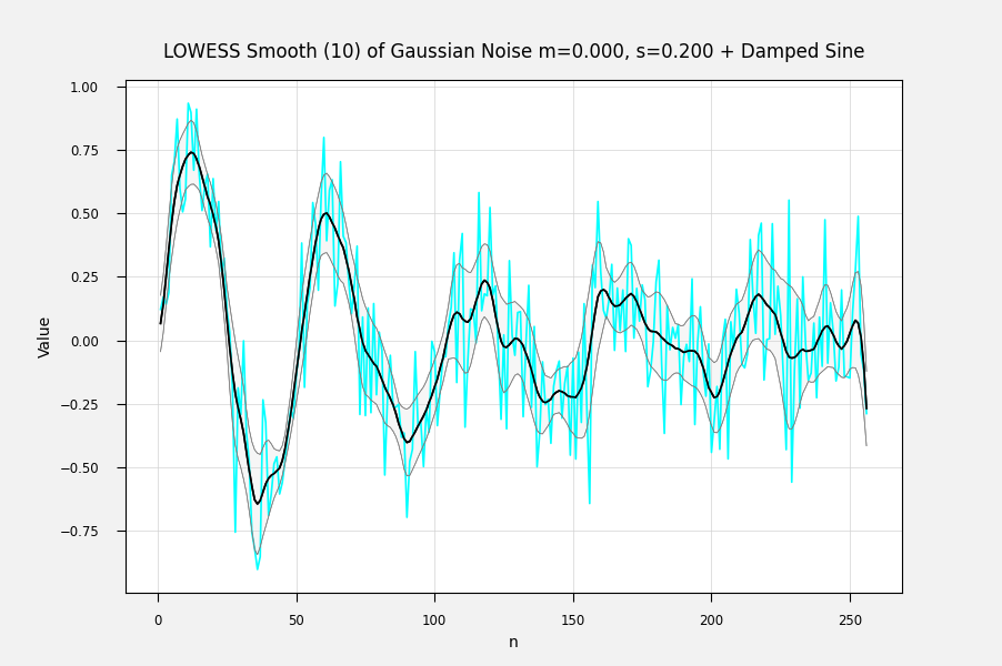
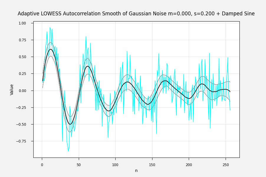
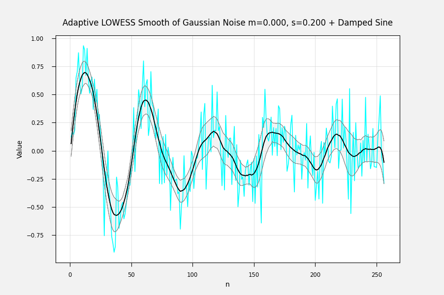
Just so. For each fitted point, its variance is the weighted sum of the squared difference from its mean:

    Svar = 0.
    for j in range(window_left, window_right):
        # ....
        Svar += wj*(yj-yfit)**2```    # wj is the weight of the j'th point in the window

    var = (Svar / Swt) *0.5*sz/(.5*sz - 1)  # sz = number of points in smoothing window

    # Approximate standard error of the fitted point
    se = ((var * Sww)**0.5) / Swt  # Swt = sum of weights, Sww = sum of squared weights

The above is from my own LOWESS brute-force (1st-degree) implementation. You can also get the correlation between the fitted points and the input data by

    e = [yfit[i] - ydata[i] for i in range(len(ydata))] # residuals
    num = 0.0
    denom = 0.0
    for i in e:
        denom += sqr(i)
    for i in range(1, len(ydata)):
        num += e[i] * e[i - 1]
    r = abs(num / denom)

Ref: p. 49 of "Nonparametric Simple Regression", J. Fox, Sage University, 2000.

IMHO, a sequence of the standard error of each point is the most useful error statistic here, because it can be used to assess the goodness of fit of different fitting procedures. The correlation can be used to condition the fit, for example by penalizing a fit for lack of smoothness.

I'm not sure how one calculates the weighted variance when the entire calculation is done with matrix methods at one go, but there must be an equation for it somewhere.

Here are some examples of fits with errorbands using the calculated standard errors. The underlying curve is a damped sine wave with normally distributed noise:

Adaptively smoothed to minimize lag-1 autocorrelation:

Adaptively smoothed with smoothness criterion:

[tbpassin]

Just to be clear, the standard error at each point is calculated from the local fitted polynomial to that point, not by simply using its deviation from the data point. The latter would only give the average variance/std error over the entire data set. The former gives the point-by-point errors, which will be more useful, for example in identifying outliers.

[sigvaldm]

Thanks for the explanation. So let's see if I got it right: all points in the original data is used for calculating each point-wise variance/standard error (except that possibly the weighting is zero for points outside the window). All points are compared to the polynomial fitted locally to the point under consideration, and then weighted by the kernel?

I believe implementing this could be a stepping stone towards the functionality mentioned in issue #4 also, right?

I guess one could leave the prediction part as it is (with the matrix and all) and then calculate the variance/standard error afterwards using a vectorized Numpy-expression, right? If you are interested in contributing to localreg, please let me know. If not, I'll keep it here in my issue-list until I find time.

[tbpassin]

Let me rephrase what I mean, because I think you mean the same thing but I'm not sure.

For each data point:

• Calculate the weighted polynomial fit over the window;
• Calculate the weighted standard deviation (sigma) over the window;
• The standard error of the fitted point equals sigma/sqrt(N), where N is the "effective" number of points in the window (probably the effective degrees of freedom, but I don't know how to compute that for a weighted window).

For my own implementation, which uses a truncated Gaussian instead of a tricube for the weights, I use an effective N of (window width) / 2. It seems to give results that agree well with the known standard errors of a linear least squares fit to a straight line.

Naturally, if there is substantial bias (e.g., a local linear fit to a sharply peaked part of the data), the sum of the squared residuals will include the bias as well as the random error, but hey, what else can you do?

For Issue #4, yes, I think it's just what is needed. One would test for outliers using the standard deviation instead of the standard error.

Numpy's poly fit can return the sum of the squared residuals of the fit, which ought to be what is needed here, but in my first explorations the size of the residuals seems way too small. Anyway, with NumPy it would be easy to compute the weighted residuals at each point if needed.

As for me contributing, I don't think I understand the linearAlg stuff well enough at this point to be too helpful. My own implementations have been brute force - ordinary algebra, not even vector/matrix methods. But for a local quadratic fit, it's easy to visibly suffer from poor conditioning, hence my interest in your localreg package.

BTW, if you want to look at it, the software I used to generate the curves I attached earlier is my GF4-project, on GitHub at

GF4 Project

GF4 has a plugin facility, and I wrote a plugin to run localreg so I could explore it. (The plugin isn't committed on the Github repo as yet).

[tbpassin]

Just to be clear, When I wrote that I didn't think I could be too helpful, I didn't mean I would become silent after this. I just meant that figuring out the linear algebra/matrix equation techniques for getting residuals, etc, would not one of my strong points. As for looking at any results to see if they might be useful, potential API changes, how to use the local residuals, those kind of things would be a better fit.

[sigvaldm]

That's completely understandable. You've already helped out, and I appreciate it :) I am quite eager about this suggestion, and would like to implement it. Realistically speaking, I don't have much time, and can make no promises when it will happen. Even so, I pay attention to the issue list, and hopefully I will find time for this one at some point.

NB: Nice project, this GF4! GF4 and Localreg complement each other well!

[tbpassin]

Thanks for the kind words! Yes, GF4 can make exploring and evaluating various techniques easy and fun in a way that just looking at printouts or summary statistics doesn't.

About APIs, my own LOWESS routine returns a list of outliers. That's easy to do because when each point is fitted, the standard deviation of the fit is also calculated. GF4 does not use this information as yet, because I have not figured out how to use it in a way that is consistent with the rest of the user interface, but other software (like localreg) could easily do so.

It's also trivial to do a Leave-One-Out fit by setting the weight at the center of the weight series to 0. This removes the focal point's value from the calculations. Nothing else has to change.

[tbpassin]

As a proof of principle, I wrote a GF4 plugin to apply Numpy's np.polynomial.polynomial.Polynomial.fit to fit each point in a dataset, and then compute the variance, etc of the fit. It's inelegant and only for the 2-D case, but at least it shows a way to do it if there isn't a clear way to do it with matrix/linear algebra methods.

Once you get the the coefficients of the weighted polynomial fit, then:

    # The fitted point:
    y0 = np.polynomial.polynomial.polyval(xdata[i], polyfit.coef)
    Svar = 0.
    Swt = 0.
    Sww = 0.
    #  x_left, x_right are the indices of the window of non-zero weights
    # (assuming compact support)
    for j in range(x_left, x_right - 1):
        weight_index = j - x_left
        wj = wt.weights[weight_index]
        xj = xdata[j]
        yj = ydata[j]
        yfit = np.polynomial.polynomial.polyval(xj, polyfit.coef)
        Svar += wj*(yj-yfit)**2
        Swt += wj
        Sww += wj*wj

    var = (Svar / Swt) *0.5*sz/(.5*sz - 1)

    # Approximate standard error of the fitted point
    se = sqrt((Svar/Swt) / ((Swt**2 / Sww) - 1))

    is_flier = (abs(ydata[i] - y0) > cliplevel * sqrt(var))

    return (y0, var, se, is_flier)

Not that localreg should compute the fit statistics this way, but this provides a baseline to compare against.