Performance comparison
Platform : Intel i7-9700K, Ubuntu x64 20.04, clang v10.00, compilation flag -O3 (all others default).
Speed measured using open source program benchHash.
| Hash Name | Width | Large Data Bandwidth (GB/s) | Small Data Velocity | Comment |
|---|---|---|---|---|
| XXH3 (SSE2) | 64 | 31.5 GB/s | 133.1 | |
| XXH128 (SSE2) | 128 | 29.6 GB/s | 118.1 | |
| RAM sequential read | N/A | 28.0 GB/s | N/A | For reference |
| City64 | 64 | 22.0 GB/s | 76.6 | |
| T1ha2 | 64 | 22.0 GB/s | 99.0 | Slightly worse collision ratio |
| City128 | 128 | 21.7 GB/s | 57.7 | |
| XXH64 | 64 | 19.4 GB/s | 71.0 | |
| SpookyHash | 64 | 19.3 GB/s | 53.2 | |
| Mum | 64 | 18.0 GB/s | 67.0 | Slightly worse collision ratio |
| XXH32 | 32 | 9.7 GB/s | 71.9 | |
| City32 | 32 | 9.1 GB/s | 66.0 | |
| SeaHash | 64 | ~7.2 GB/s | ??? | estimated from a different run |
| Murmur3 | 32 | 3.9 GB/s | 56.1 | |
| SipHash | 64 | 3.0 GB/s | 43.2 | |
| Blake3 (SSE2) | 256 | 2.4 GB/s | 8.1 | Cryptographic |
| HighwayHash | 64 | 1.4 GB/s | 6.0 | |
| FNV64 | 64 | 1.2 GB/s | 62.7 | Poor avalanche properties |
| Blake2 | 256 | 1.1 GB/s | 5.1 | Cryptographic |
| Blake3 portable | 256 | 1.0 GB/s | 8.1 | Cryptographic |
| SHA1 | 160 | 0.8 GB/s | 5.6 | No longer cryptographic (broken) |
| MD5 | 128 | 0.6 GB/s | 7.8 | No longer cryptographic (broken) |
| SHA256 | 256 | 0.3 GB/s | 3.2 | Cryptographic |
Note : Small data velocity is a rough average of algorithm's efficiency for small data. For more accurate information, please refer to graphs in second part below.
The following algorithms run on modern x64 cpus, but are either not portable, or their performance depend on the presence of a non-guaranteed instruction set (note: only SSE2 is guaranteed on x64).
Benchmark system is identical, but compilation flags are now -O3 -mavx2.
| Hash Name | Width | Large Data Bandwidth (GB/s) | Small Data Velocity | Comment |
|---|---|---|---|---|
| XXH3 (AVX2) | 64 | 59.4 GB/s | 133.1 | AVX2 support (optional) |
| MeowHash (AES) | 128 | 58.2 GB/s | 52.5 | Requires x64 + hardware AES (not portable) |
| XXH128 (AVX2) | 128 | 57.9 GB/s | 118.1 | AVX2 support (optional) |
| CLHash | 64 | 37.1 GB/s | 58.1 | Requires PCLMUL intrinsics (not portable) |
| RAM sequential read | N/A | 28.0 GB/s | N/A | For reference |
| ahash (AES) | 64 | 22.5 GB/s | 107.2 | Hardware AES, results vary depending on instruction set and version |
| FarmHash | 64 | 21.3 GB/s | 71.9 | Results vary depending on instruction set |
| CRC32C (hw) | 32 | 13.0 GB/s | 57.9 | Requires SSE4.2 |
| Blake3 (AVX2) | 256 | 4.4 GB/s | 8.1 | AVX2 support (optional) |
CRC32C can be done in software, but performance becomes drastically slower.
XXH3 and XXH128 and Blake3 can also use AVX512, but this instruction set is not available on test platform.
Note : some algorithms are effectively faster than system's RAM. Their full speed can only be leveraged when hashing data segments already present in cache.

It's interesting to note that the layers of caches are clearly visible in the graph. The host cpu has an L1 cache of 32 KB, L2 cache of 256 KB, and L3 cache of 12 MB. Performance of the AVX2 variant visibly plummets on passing each of these thresholds.
So far, we have looked at 64-bit performance, where 64-bit hashes have an advantage, if only by virtue of ingesting data faster. The situation changes drastically on 32-bit systems, as emulating 64-bit arithmetic on 32-bit instruction set takes a big toll on performance.
The following graph shows how these hash algorithms fare in 32-bit mode. Most of them suffer a large decrease in performance. Only 32-bit hashes maintain their performance, like XXH32. But good news is, XXH3 is also good on 32-bit cpus, and even more so when a vector unit is available.

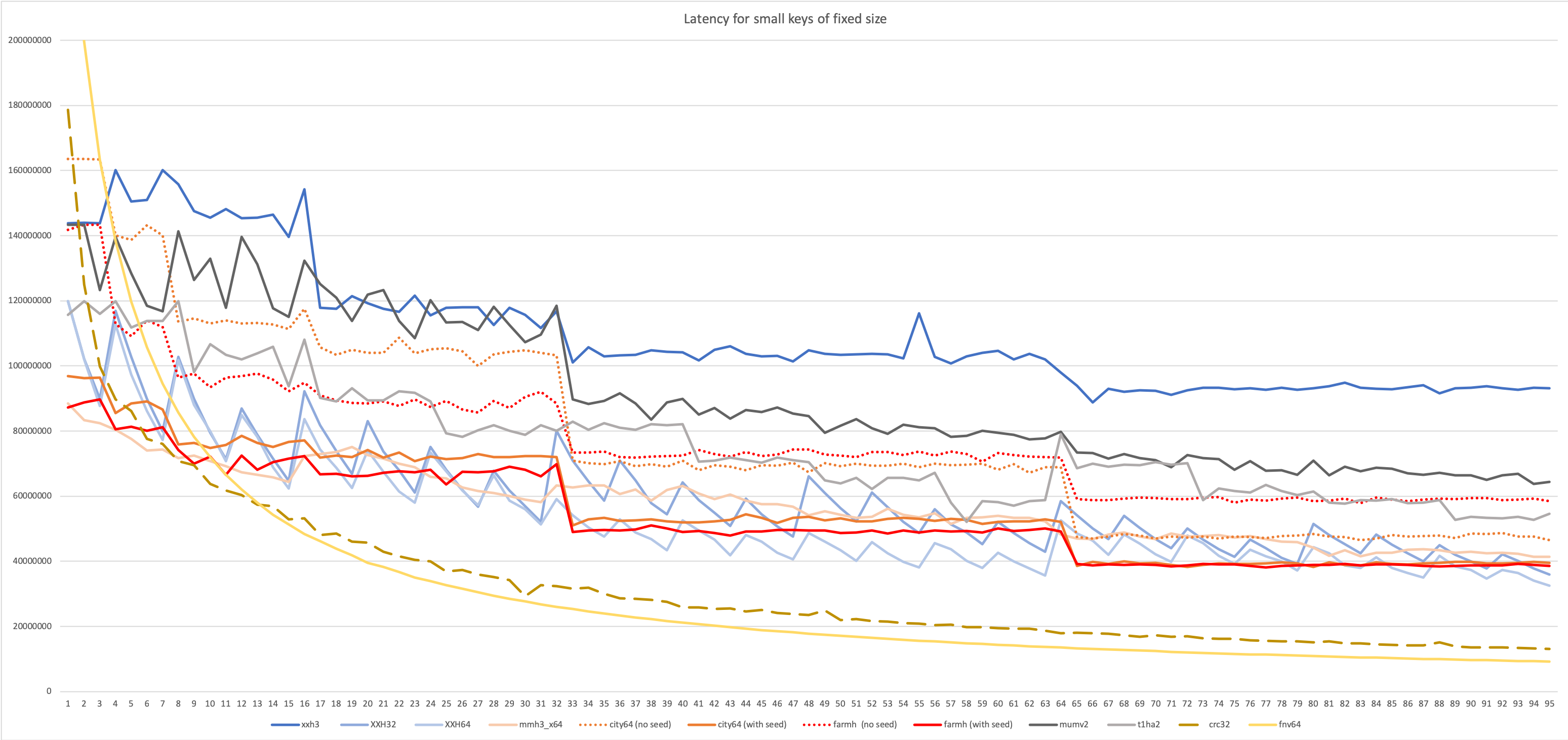
In many use cases, the generated hash value can be used to populate a hash table or a bloom filter. In these scenarios, it's frequent that the hash algorithm is just a part of a larger system, such as a database, and it will be invoked for a lot of rather small objects. When hashing small objects, hash properties can vary vastly compared to hashing "large" inputs. Some algorithms, for example, may have a long start or end stages, becoming dominant for small inputs. The below tests try to capture these characteristics.
Throughput tests try to generate as many hashes as possible. This is classically what is measured, because it's the easiest methodology for benchmark. However, it is only representative of "batch mode" scenarios, and also requires all inputs to feature exactly the same length. So it's effectively not that representative at all.

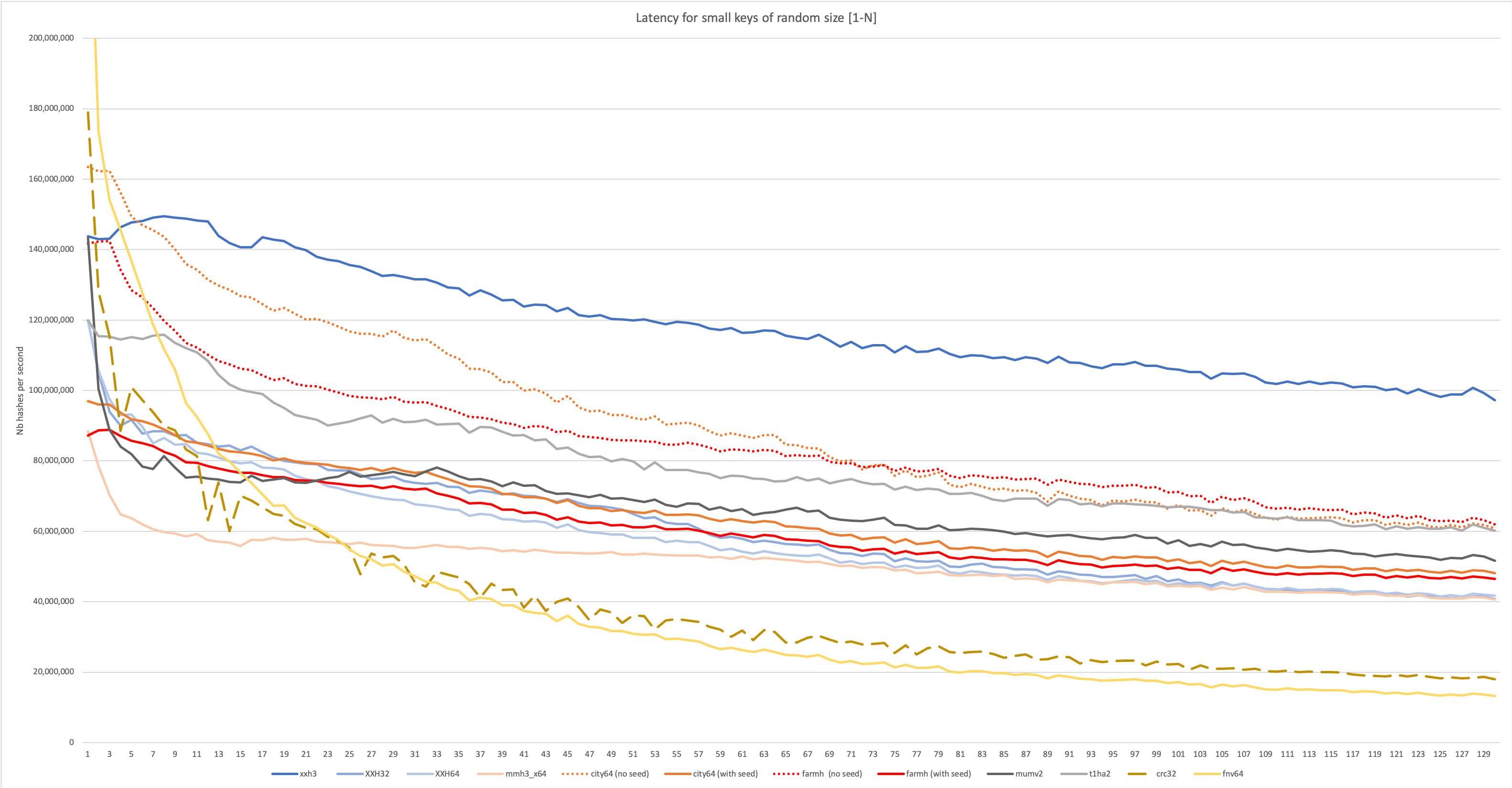
In this more advanced scenario, input length is not longer stable. This situation is generally more common, so the scenario is more likely to be representative of some real use case. However, being a throughput test, it's still targeting batch-mode scenarios, where a lot of hashes must be produced repetitively. In the graph below, length is effectively random, read from a generated series of value between 1 and N. This situation is much harder on the branch predictor, which is likely to miss quite a few guesses, occasionally triggering a pipeline flush. Such negative impact can quickly dominate performance for small input. Some algorithm are better design to resist this side-effect.

Latency tests require the algorithm to complete one hash before starting the next one. This is generally more representative of situations where the hash is integrated into a larger algorithm.