Hi! I'm Jeremie and this is my first attempt at making a neural network from scratch. If you want to learn about neural networks yourself, you can watch these videos. If you want to play around with making one yourself, feel free to edit, tinker and destroy my code!
This code was written in Python 3.71, and requires numpy and matplotlib. Simply run the following commands to install them:
pip install numpy
pip install matplotlib
You will need to clone this repo (rather than download the ZIP) if you want it to work with the MNIST files provided, since they are managed by github lfs (large file system).
Start by creating a neural_net instance and pass in a shape for the network. The shape is a tuple with each value representing the number of nodes in that layer, including both input and output layers.
# This takes in 28 by 28 images, passes them through 2 hidden layers of 16 nodes, then outputs 10 values
nn = neural_network((28 * 28, 16, 16, 10))
The neural net is now initialised with random weights and biases, so in order to train it you can back-propogate training data. Make sure you only pass in batches of 10 to 100 training examples, you can re-run backprop as many times as you want and it will continue to improve.
# This will backproagate the network on the first 100 training examples
nn.backprop(training_data[:100])

# This will backproagate the network on the next 100 training examples
nn.backprop(training_data[100:200])
You can run the network with a single example.
# show=True will print the result of the final layer
nn.run(image, show=True)
You can test the performance of the network using accuracy() or loss().
# This will print the average loss over the first 200 training examples
print("Loss:", nn.loss(training_data[:200]))

# This will print the accuracy over the testing data set
print("Accuracy:", str(nn.test(testing_data) * 100) + "%")
You might be wondering why you needed to install matplotlib, well here's your answer! You can display the weights of your network as images to gain an understanding about how it works internally. For these to work well, try to use square numbers for the number of nodes in each layer of your network.
# This will show the weights for each node in the first hidden layer
nn.show()

# This will show the weights for each node in the second hidden layer
nn.show(2)
Here is what the first layer of an untrained network looks like:
You can also display an example of your training data like so:
# This will show the handwritten digit 5
img_show(training_data[0][0])
A big part of machine learning and in particular neural networks is maths, specifically linear algebra and multi-variable calculus. Here I will try to explain the maths behind my code to demystify some of the more complicated parts. I do encourage you to watch the video series I linked to in the intro.
The easiest part is simply running the network, here I'll define some notation to make things easier. The nth layers' weights, biases and activations are defined like this respectively:
The operation of going from one layer to the next is where the linear algebra applies, and it's as follows:
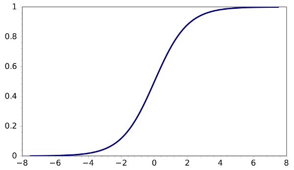
That funny symbol represents the sigmoid function which squishes all numbers on the number line between 0 and 1.
Finally we take the output layer y, and use it to calculate a loss based on the true answer:
Now the hard stuff. So we want to find the derivative of Loss with respect to every weight and bias in the network, but we can use the chain rule to make this a bit easier.


