This project aims to develop a Machine Learning model to classify and label various barbell exercises using accelerometer and gyroscope data obtained using a Metamotion sensor.
Once fully functional, this project could serve as the foundation for a versatile fitness application where the users exercises are classified and recorded. Additionally a method of counting repetitions could also be implimented.
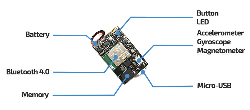
The Metamotion sensor provides comprehensive data, including gyroscope, accelerometer, magnetometer, sensor fusion, barometric pressure, and ambient light.
We only require the raw accelerometer and gyroscope data.
- Overview
- Data Collection
- Python Scripts
- Data Visualization
- Outlier Detection & Management
- Feature Engineering
- Predictive Modelling
The provided dataset, available in the metamotion.zip file ('data/raw'), contains gyroscope and accelerometer data for heavy and light barbell movements. Data is collected for all three axes for both gyroscopes and accelerometers, including rest data. It contains a weeks worth of data from various participants all doing the same exercises with varying degrees of execution.
its important to note that the gyroscope recorded data at a greater frequency than the accelerometer.
Accelerometer:    12.500HZ
Gyroscope:        25.000Hz
- Bench (bench)
- Squat (squat)
- Barbell Overhead Press (OHP)
- Deadlift (dead)
- Barbell Row (row)
make_dataset.py: (src/data) - Contains code used to extract and transform the original raw data.visualize.py: (src/visualization) - Includes code for generating various visualizations from the preprocessed sensor data.remove_outliers.py: (src/features) - Implements outlier detection methods and removes outliers from the dataset.build_features.py: (src/features) - Implements feature engineering steps such as handling missing values, calculating set duration, applying a Butterworth lowpass filter, conducting principal component analysis (PCA), computing sum of squares attributes, and performing temporal abstraction.train_model.py: (src/model) - Defines and trains predictive models using the selected machine learning algorithms to perform multiclass classification on the sensor data.
DataTransformation.py: (src/features) - Provides functions and classes for data transformation tasks such as low-pass filtering and principal component analysis.TemporalAbstraction.py: (src/features) - Implements functions and classes for temporal abstraction tasks, facilitating the computation of rolling averages (means) and standard deviations for sensor measurements over specified windows.FrequencyAbstraction.py: (src/features) - Performs Fourier transformations on the data to identify frequencies and filter noise, adding frequency-related features to the dataset for further analysis and modeling tasks.LearningAlgorithms.py: (src/model) - Contains implementations of various machine learning algorithms for classification tasks, including k-nearest neighbors, decision trees, random forest, support vector machines, and feedforward neural networks.
filepath : src\data\make_dataset.py
The gyroscope and accelerometer raw data files within the MetaMotion folder are named as follows:
# Accelerometer:
"../../data/raw/MetaMotion/A-bench-heavy2-rpe8_MetaWear_2019-01-11T16.10.08.270_C42732BE255C_Accelerometer_12.500Hz_1.4.4.csv"

#Gyroscope:
../../data/raw/MetaMotion/A-bench-heavy2-rpe8_MetaWear_2019-01-11T16.10.08.270_C42732BE255C_Gyroscope_25.000Hz_1.4.4.csv
The file naming convention prominently includes several key components: a participant identifier (A), an exercise label (bench), a category descriptor (heavy), and supplementary details like RPE (rate of perceived exertion).
To initiate the extraction of information from the file path and name, refer to the code snippet below:
files = glob("../../data/raw/MetaMotion/*.csv")
print(files)
This returns:
['../../data/raw/MetaMotion\\A-bench-heavy2-rpe8_MetaWear_2019-01-11T16.10.08.270_C42732BE255C_Accelerometer_12.500Hz_1.4.4.csv',...]
Here we have already encountered my first issue, the filepath returned now contains \\ instead of /
which will cause an issue when trying to .split .
for file in files:

    filename = file.replace("\\", "/")
The simple replacement above will now allow us to split the filename and extract participant, exercise and category.
The re regular expressions module was used to remove the _MetaWear_ and any numerical values:
    participant = filename.split("/")[-1].split("-")[0]
    exercise = filename.split("/")[-1].split("-")[1]
    category = filename.split("/")[-1].split("-")[2]
    category = re.sub(r"\d+|_MetaWear_", "", category)
participant, exercise, category have been extracted.
By reading the file into a dataframe we can then create appropriately named columns to store the extracted variables:
    df = pd.read_csv(file)
        df["participant"] = participant
        df["exercise"] = exercise
        df["category"] = category
The initialization of two empty dataframes and two variables depicted below serves the purpose of concatenating all dataframes into the corresponding ones and generating a unique identifier, "set," for each data file. These elements will be pre-set before the aforementioned for loop
acc_df = pd.DataFrame()
gyr_df = pd.DataFrame()

acc_set = 1
gyr_set = 1
Based on the filename, we generate the set column in the dataframe and populate it using the corresponding set variable (acc_set or gyr_set). Subsequently, we concatenate this updated dataframe with the existing Accelerometer (acc_df) or Gyroscope (gyr_df) dataframes.
Throughout the loop iterating over all files, these two dataframes will continuously update and expand.
    if "Accelerometer" in file:
        df["set"] = acc_set
        acc_set += 1
        acc_df = pd.concat([acc_df, df])

    if "Gyroscope" in file:
        df["set"] = gyr_set
        gyr_set += 1
        gyr_df = pd.concat([gyr_df, df])
Creating a new epoch (ms) column, assigning as the index and converting from Unix to datetime in the units 'ms'.
acc_df.index = pd.to_datetime(acc_df["epoch (ms)"], unit="ms")
gyr_df.index = pd.to_datetime(gyr_df["epoch (ms)"], unit="ms")
Pruned unnecessary columns:
del acc_df["epoch (ms)"]
del acc_df["time (01:00)"]
del acc_df["elapsed (s)"]

del gyr_df["epoch (ms)"]
del gyr_df["time (01:00)"]
del gyr_df["elapsed (s)"]
Merging acc_df and gyr_df into one dataframe merged_df:
merged_df = pd.concat([acc_df.iloc[:, :3], gyr_df], axis=1)
Renaming columns so the dataframe is easier to understand at a glance:
merged_df.columns = [
    "acc_x",
    "acc_y",
    "acc_z",
    "gyr_x",
    "gyr_y",
    "gyr_z",
    "label",
    "exercise",
    "category",
    "set",
]
After merging our dataframes, we observe that numerous rows exclusively contain gyroscope data, others exclusively accelerometer data, while only a few include both.
This disparity arises from the gyroscope sensor's higher recording frequency compared to the accelerometer sensor. Consequently, instances of both sensors capturing data simultaneously are rare.
To enhance the completeness of our dataset, we propose resampling the data using aggregation methods such as mean for numerical values and last for non-numeric ones. This approach leverages the time-series nature of our data, enabling us to consolidate and fill in missing values effectively.
aggregation_method = {
    "acc_y": "mean",
    "acc_x": "mean",
    "acc_z": "mean",
    "gyr_x": "mean",
    "gyr_y": "mean",
    "gyr_z": "mean",
    "label": "last",
    "exercise": "last",
    "category": "last",
    "set": "last",
}
Before applying the resampling methods described above, it's crucial to acknowledge that we're working with time-series data. Resampling the entire merged_df without consideration would lead to an excessive number of null rows. Given that the data spans a week in terms of time series, and considering it was collected only for short durations each day, a direct resampling approach would generate impractical amounts of missing values.
Instead of resampling the entire dataset at once, the dataset is split into smaller groups based on daily intervals. This reduces the computational burden of the resampling operation:
days = [g for n, g in merged_df.groupby(pd.Grouper(freq="D"))]
Resampling at a frequency of 200 milliseconds appeared to retain a significant number of rows and produce a more comprehensive dataframe named data_resampled.
data_resampled = pd.concat([df.resample(rule="200ms").apply(aggregation_method).dropna() for df in days])
data_resampled["set"] = data_resampled["set"].astype("int")
Exporting data to a pickle file is a versatile and efficient solution for storing and exchanging serialized data in Python, offering advantages in terms of serialization efficiency, data preservation, compatibility, ease of use, and support for compression.
data_resampled.to_pickle("../../data/interim/01_data_processed.pkl")
filepath : src\visualization\visualize.py
In this section, we explore sensor data visualizations to gain crucial insights into exercise patterns and participant behaviour, enhancing our machine learning model. These visuals offer a comprehensive understanding of the data dynamics,
We compare medium vs. heavy sets for a specific exercise, such as squats:
fig, ax = plt.subplots()
category_df.groupby(['category'])['acc_y'].plot()
ax.set_ylabel("acc_y")
ax.set_xlabel ("samples")
plt.legend()
plt.savefig("../../reports/figures/Squat_A_Heavy_Medium.png")
Resulting plot:
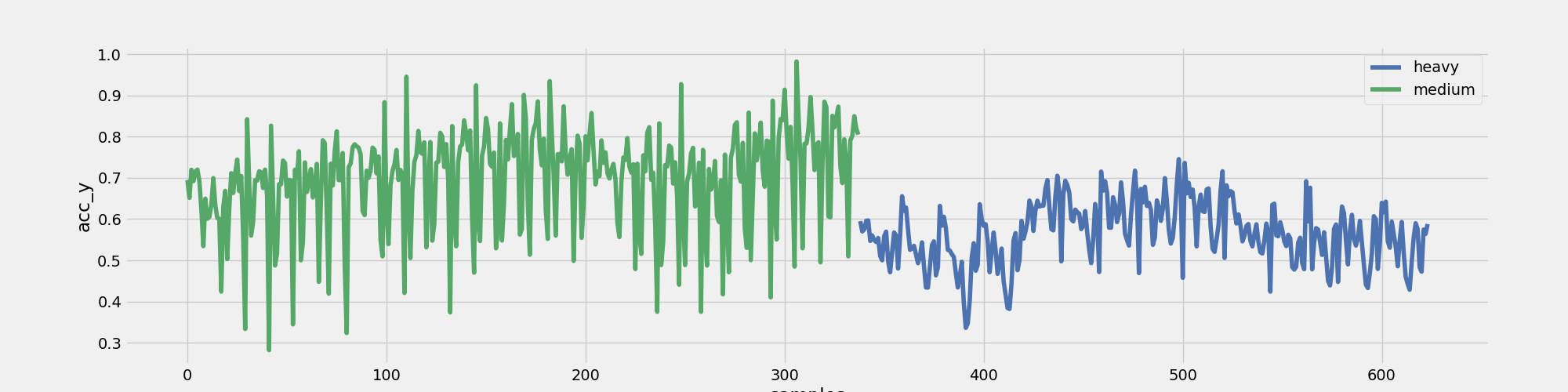 Figure 1: Participant A Squats - Heavy/Medium - No of Samples vs Accelerometer (y-axis)
Figure 1 indicates that Participant A exhibited reduced acceleration along the y-axis when training with a heavy weight compared to a medium weight. While this outcome was anticipated, it's reassuring to see that our data aligns with this expectation.
Here's where things get interesting:
for label in labels:
    for participant in participants:
        all_axis_df = df.query(f"label == '{label}'").query(f"participant == '{participant}'").reset_index()
        if len(all_axis_df) > 0:
            fig, ax = plt.subplots(nrows=2, sharex=True, figsize=(20,10))
            all_axis_df[["acc_x","acc_y","acc_z"]].plot(ax=ax[0])
            all_axis_df[["gyr_x","gyr_y","gyr_z"]].plot(ax=ax[1])

            ax[0].legend(loc='upper center', bbox_to_anchor=(0.5,1.15),ncol=3,fancybox=True,shadow=True)
            ax[1].legend(loc='upper center', bbox_to_anchor=(0.5,1.15),ncol=3,fancybox=True,shadow=True)
            ax[1].set_xlabel('samples')

            plt.savefig(f"../../reports/figures/{label.title()} ({participant}).png")
            plt.show()
The for loop generates a series of figures which we can help with:
Comparative Analysis: By comparing accelerometer and gyroscope data between different exercises and participants, we can identify patterns and variations in movement. This aids in selecting relevant features for the model and understanding how different factors influence the sensor data.
Insights into Movement: Understanding movement patterns and characteristics helps in feature engineering. By extracting relevant features from the sensor data, we can provide the model with meaningful input that captures important aspects of exercise performance.
Anomaly Detection: Detecting anomalies in the sensor data helps in data preprocessing and quality control. By identifying and addressing irregularities, we ensure that the input data for the machine learning model is clean, accurate, and representative of typical exercise performance. This enhances the model's ability to generalize and make accurate predictions.
.png) Figure 2: Participant B Bench Press - plot displaying accelerometer and gyroscope data in all three axis (x,y,z).
Figure 2: Participant B Bench Press - plot displaying accelerometer and gyroscope data in all three axis (x,y,z).
.png) Figure 3: Participant D Bench Press - plot displaying accelerometer and gyroscope data in all three axis/planes (x,y,z).
Figure 3: Participant D Bench Press - plot displaying accelerometer and gyroscope data in all three axis/planes (x,y,z).
In both Figure 2 and Figure 3, it's noticeable that despite both participants performing the same exercise, there are considerable differences in the gyroscope data and acc_y plots. These disparities may stem from variations in bench press execution, such as differences in form, rep control, and speed. However, across all Bench Plots from all participants, there's a consistent observation of minimal acceleration in the x and z plane and maximal acceleration in the y plane.
filepath : src\features\remove_outliers.py
We visualise the outliers from our data/interim/01_data_processed.pkl file, using box plots and histograms to understand their distribution across different exercises and participants.
To detect outliers, we implement three different methods: interquartile range (IQR), Chauvenet's criterion, and Local Outlier Factor (LOF). After evaluating these methods.
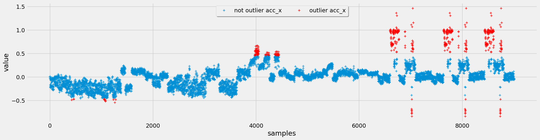
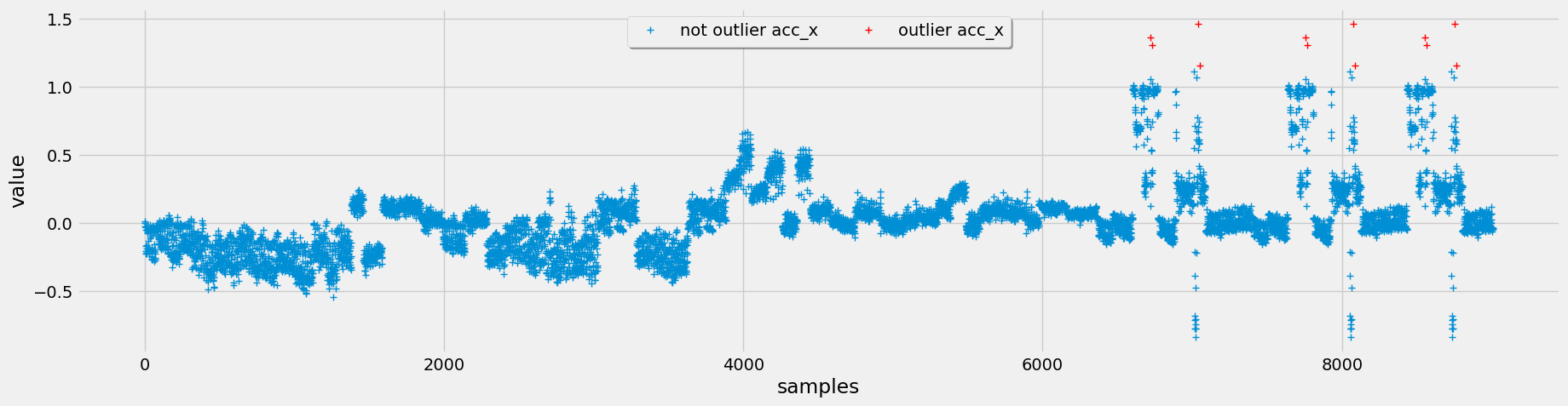
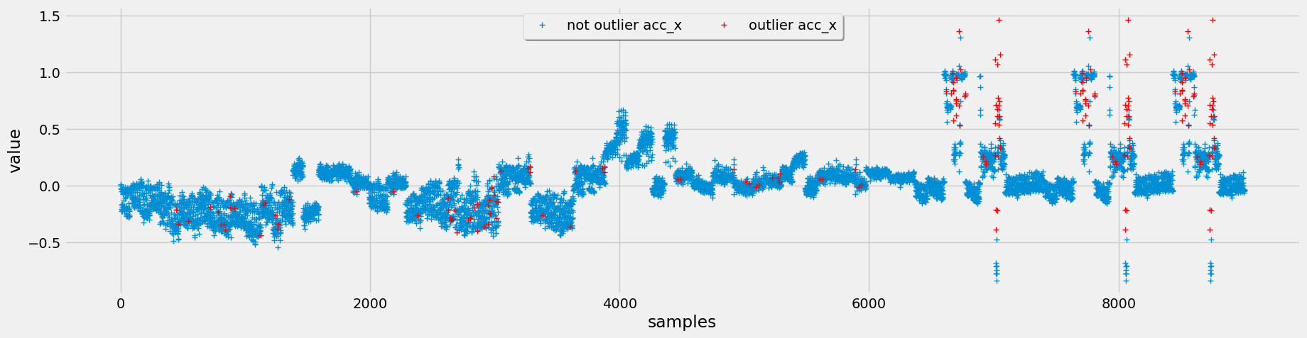 Figure 4: Top (IQR Outlier Detection), Middle (Chauvenet Outlier Detection), Bottom (LOF Outlier Detection)
Opting for Chauvenet's criterion for outlier detection, we leverage its assumption of a normal distribution, which aligns well with our data characteristics. Additionally, it tends to flag fewer outliers, but those identified are more pertinent to our analysis.
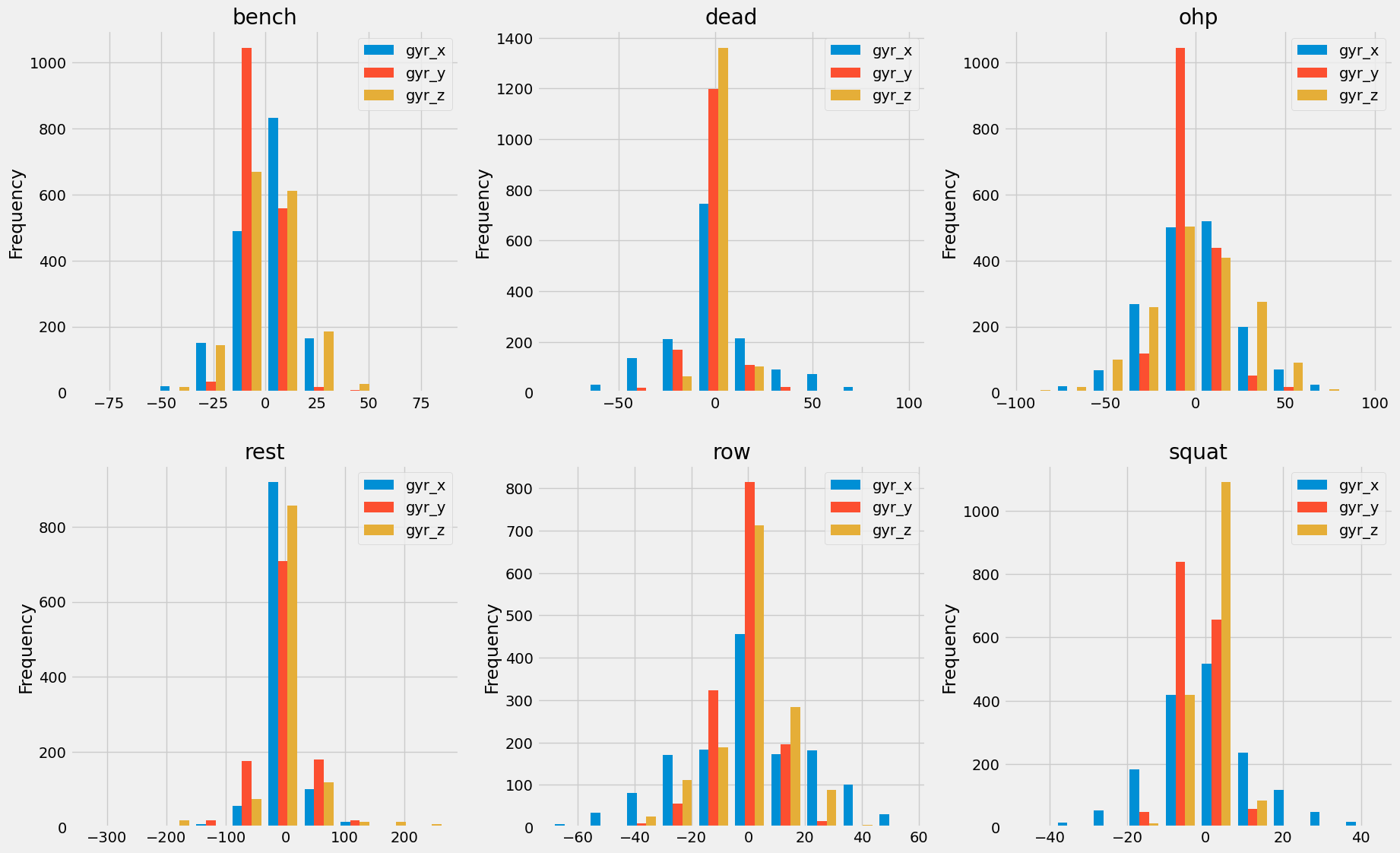 Figure 5: Exercise gyroscope data showing normal distribution characteristics
Chauvenet's criterion identifies outliers based on the assumption of a normal distribution, making it suitable for our sensor data analysis. We apply this method to each sensor's data columns, marking outliers and subsequently replacing them with NaN values. This approach ensures that the machine learning model isn't skewed by anomalous data points, leading to more robust and accurate predictions.
Finally, we export the cleaned dataset with outliers removed, ready for further preprocessing and model development.
see file: data\interim\02_outliers_removed_chauvenets.pkl
filepath : src\features\build_features.py
This section outlines the feature engineering pipeline used to preprocess the sensor data for exercise classification. The analysis involves various stages, including handling missing values, filtering, dimensionality reduction, and extracting relevant features.
Missing values in the dataset are handled through linear interpolation to ensure continuity in the time series data using the for loop below:
for col in predictor_columns:
    df[col] = df[col].interpolate()
Where:
df = pd.read_pickle("../../data/interim/02_outliers_removed_chauvenets.pkl")

predictor_columns = list(df.columns[:6])
Interpolation/Imputation Visualized:
.png) Figure 6: gyr_y data plot for set 35 Overhead Press, pre interpolation.
Figure 6: gyr_y data plot for set 35 Overhead Press, pre interpolation.
.png) Figure 7: gyr_y data plot for set 35 Overhead Press, post interpolation.
Figure 7: gyr_y data plot for set 35 Overhead Press, post interpolation.
The duration of each exercise set is calculated to provide insights into the length of time spent on each exercise.
for s in df["set"].unique():
    start = df[df["set"]== s].index[0]
    stop = df[df["set"]== s].index[-1]

    duration = stop - start
    df.loc[(df["set"] == s), "duration"] = duration.seconds

duration_df = df.groupby(["category"])["duration"].mean()
duration_df.iloc[0] / 5 #5 heavy reps
duration_df.iloc[1] / 10 #10 medium reps
The code above computes the duration of each exercise set by subtracting the start time from the stop time. It then calculates the average duration for each exercise category. This helps in understanding the typical time taken for sets and repetitions, facilitating performance assessment and training optimization.
Returning:
category
heavy       14.743501
medium      24.942529
sitting     33.000000
standing    39.000000
Name: duration, dtype: float64
df_lowpass = df.copy()
LowPass = LowPassFilter()

s_freq = 1000 / 200 #200 ms : 5 instances per second
cutoff_freq = 1.3

for col in predictor_columns:
    df_lowpass = LowPass.low_pass_filter(df_lowpass, col , s_freq,cutoff_freq, order=5)
    df_lowpass[col] = df_lowpass[col + "_lowpass"]
    del df_lowpass[col + "_lowpass"]
The code snippet provided is utilizing the LowPassFilter class from the DataTransformation module (DataTransformation.py) to perform the lowpass filtering operation on the accelerometer and gyroscope data.
 Figure 8: Application of Butterworth Low Pass Filter.
The code applies a Butterworth lowpass filter to the accelerometer and gyroscope data in order to remove high-frequency noise while preserving the underlying signal trends.
The cutoff frequency of the filter is chosen to attenuate frequencies above a certain threshold, effectively smoothing out rapid fluctuations in the data. This is particularly useful for motion sensor data, where high-frequency noise can obscure meaningful patterns and introduce inaccuracies in analysis.
The filtered data (df_lowpass) is then used for further analysis, ensuring that subsequent calculations and visualizations are based on a cleaner representation of the original sensor measurements.
The application of PCA on df_lowpass begins with determining the explained variance for each principal component, providing insight into how much of the original data's variability is captured by each component.
The code snippet below is utilizing the PrincipalComponentAnalysis class from the DataTransformation module (DataTransformation.py)
df_pca = df_lowpass.copy()
PCA = PrincipalComponentAnalysis()

pca_values = PCA.determine_pc_explained_variance(df_pca, predictor_columns)
Using the elbow method, the optimal number of principal components to retain is identified see figure 8, balancing dimensionality reduction with information retention.
plt.figure(figsize = (10,10))
plt.plot(range(1, len(predictor_columns) + 1), pca_values)
plt.xlabel("principal component number")
plt.ylabel("explained variance")
plt.show()
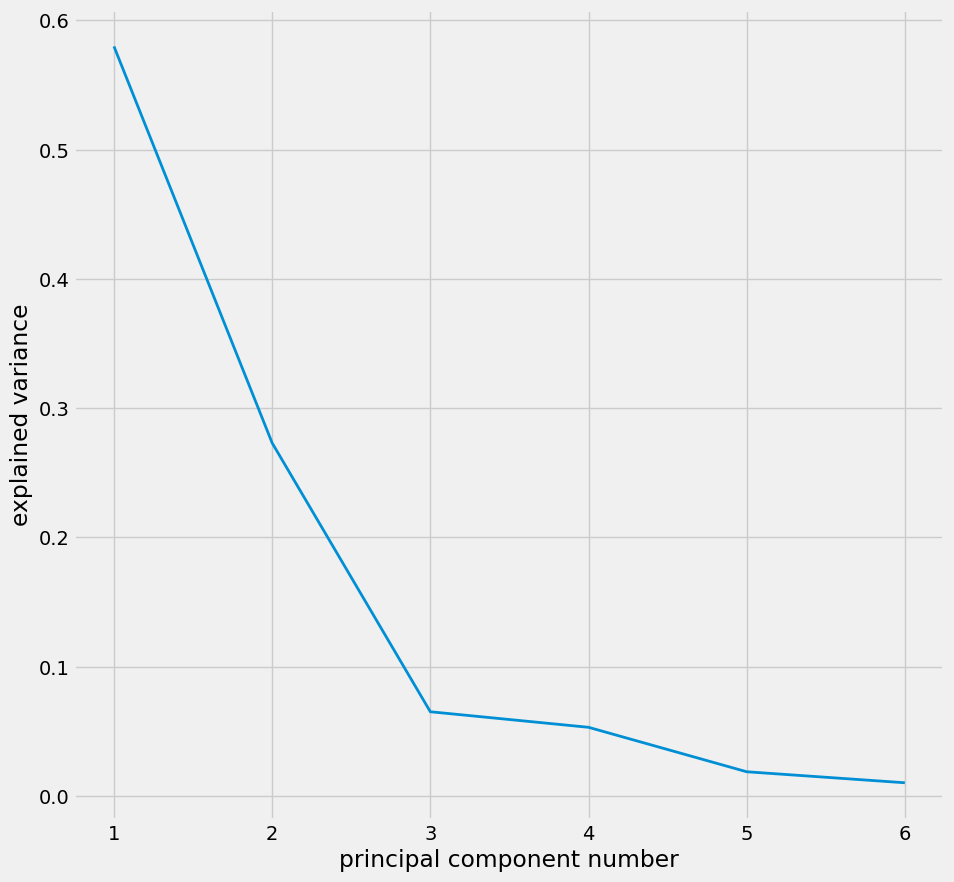 Figure 9: Plot identifies the optimal number of components as 3.
df_pca = PCA.apply_pca(df_pca,predictor_columns,3)
Subsequently, PCA is applied to transform the dataset into a lower-dimensional space while preserving most of its variability.
subset = df_pca[df_pca["set"] == 35]
subset[["pca_1", "pca_2", "pca_3"]].plot()
This transformation allows for the representation of the data along orthogonal directions, facilitating efficient computation and visualization.
The transformed data is visualized in Figure 10 and 11 to understand the patterns and structure captured by the principal components, aiding in further analysis and interpretation of the dataset.
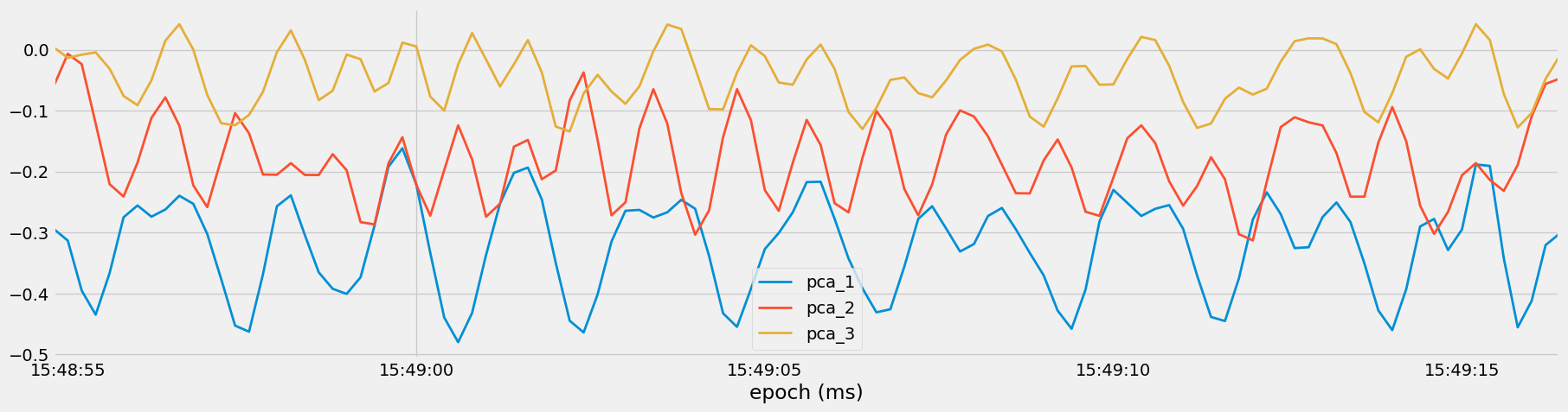 Figure 10: Visualization of Principal Components for Set 35, Medium Overhead Press.
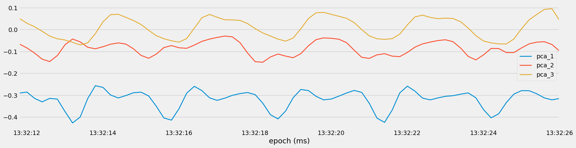 Figure 11: Visualization of Principal Components for Set 40, Heavy Bench.
df_squared = df_pca.copy()

acc_r = df_squared["acc_x"] ** 2 + df_squared["acc_y"] ** 2 + df_squared["acc_z"] ** 2
gyr_r = df_squared["gyr_x"] ** 2 + df_squared["gyr_y"] ** 2 + df_squared["gyr_z"] ** 2

df_squared["acc_r"] = np.sqrt(acc_r)
df_squared["gyr_r"] = np.sqrt(gyr_r)
The sum of squares attributes involves computing the magnitude of acceleration (acc_r) and angular velocity (gyr_r) vectors by summing the squares of their individual components and then taking the square root of the sum.
By computing these sums of squares attributes, we obtain scalar values representing the overall intensity of acceleration and angular velocity experienced by the sensor, irrespective of direction. These attributes provide a concise representation of the sensor data's dynamics, facilitating further analysis, visualization and feature extraction for machine learning tasks.
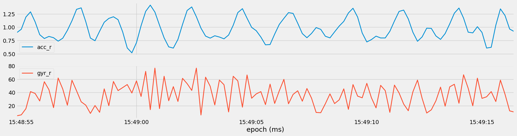 Figure 12: Visualization of the magnitude of acceleration (
acc_r) and angular velocity (gyr_r) vectors for Set 35, Medium Overhead Press.
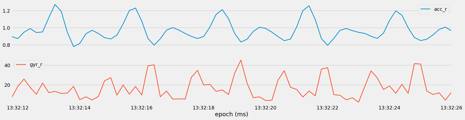 Figure 13: Visualization of the magnitude of acceleration (
acc_r) and angular velocity (gyr_r) vectors for Set 40, Heavy Bench.
The benefits of employing temporal abstraction techniques, such as computing rolling averages and standard deviations, include capturing temporal trends, smoothing noisy data, highlighting variability, facilitating feature engineering, and aiding interpretability.
This step is crucial for understanding how sensor measurements evolve over time, providing insights into patterns and behaviors that may be indicative of different exercises or states.
This approach may introduce missing data due to windowing, but it's considered an acceptable trade-off because it helps reveal underlying patterns and trends in the data, which can lead to better insights and more accurate modeling.
df_temporal = df_squared.copy()
NumAbstract = NumericalAbstraction()

predictor_columns = predictor_columns + ["acc_r","gyr_r"]
ws = int(1000 / 200) #window size of 5 to get a window of 1 second
df_temporal_list = []

for s in df_temporal["set"].unique():
    subset = df_temporal[df_temporal["set"] == s].copy()
    for col in predictor_columns:
        subset = NumAbstract.abstract_numerical(subset, [col], ws, "mean")
        subset = NumAbstract.abstract_numerical(subset, [col], ws, "std")
    df_temporal_list.append(subset)

df_temporal = pd.concat(df_temporal_list)

subset[["acc_y","acc_y_temp_mean_ws_5", "acc_y_temp_std_ws_5"]].plot()
subset[["gyr_y","gyr_y_temp_mean_ws_5", "gyr_y_temp_std_ws_5"]].plot()
The code segment computes rolling averages (means) and standard deviations for sensor measurement columns in the dataset df_squared using temporal abstraction.
It begins by creating a copy of the dataset and initializing the NumericalAbstraction class located in TemporalAbstraction.py. The window size for rolling computations is determined based on the data's sampling frequency (five samples in one second).
Then, for each unique set in the dataset, the code calculates rolling mean and standard deviation for each sensor measurement column within the set.
These values are stored in new columns added to the dataset. Due to the window size of 5, the initial four values in each rolling computation are NaN because there isn't enough preceding data.
Finally, a subset of the dataset is chosen for visualization, plotting the original sensor measurements alongside their rolling mean and standard deviation values to reveal temporal trends and variability.
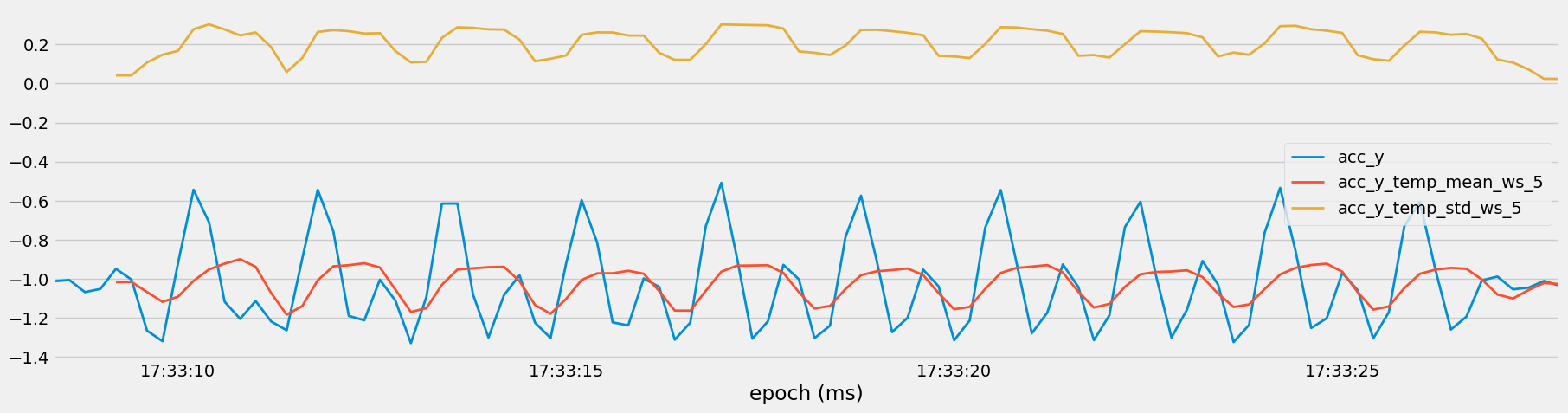
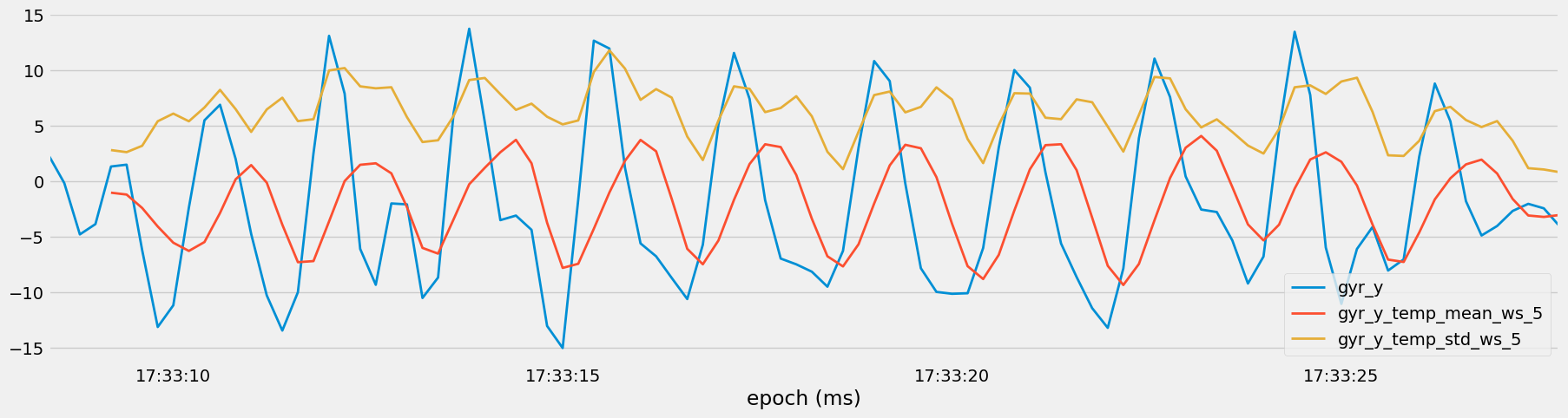 Figure 14: Temporal Trends in Sensor Measurements with Rolling Averages and Standard Deviations
The FrequencyAbstraction.py module contains the following functions:
find_fft_transformation Function: This function computes the Fourier transformation of the input data utilizing the Fast Fourier Transform (FFT) algorithm. It returns the amplitudes of both the real and imaginary components of the transformation.
abstract_frequency Function: This function derives frequency features over a specified window size for the provided columns in the dataset. It calculates several frequency-related metrics for each column, including maximum frequency, frequency-weighted value, and Power Spectral Entropy (PSE).
These transformations enable the analysis of periodic patterns and frequencies present in the sensor data.
By abstracting frequency-domain features such as maximum frequency, frequency-weighted values, and power spectral entropy, the code aims to capture underlying rhythmic patterns or oscillations within the sensor signals.
-
Max Frequency: Identifies the dominant frequency component within the specified window.
-
Frequency Weighted: Computes the weighted average of frequencies based on their corresponding amplitudes.
-
Power Spectral Entropy (PSE): Measures the complexity or randomness of the frequency distribution.
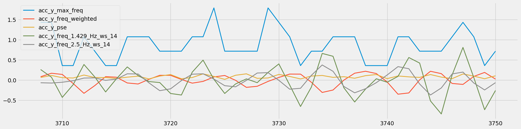
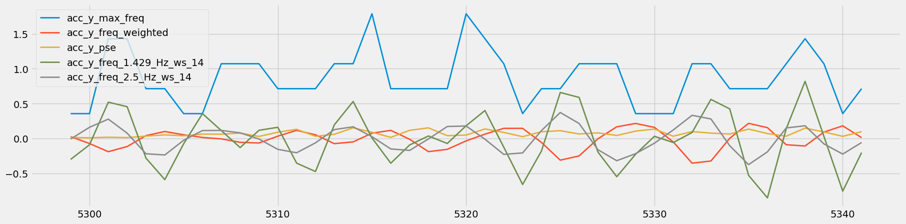 Figure 15: Visual Comparison of Heavy Rows - Sets 83 and 84
These features can be highly informative for tasks such as activity recognition or anomaly detection, as they reveal characteristic frequency components associated with different activities or states.
Overlapping windows is a common concern in time-series analysis that can lead to overfitting in subsequent modeling tasks.
df_freq = df_freq.dropna()
df_freq = df_freq.iloc[::2]
By dropping rows containing NA values and reducing overlap in the dataset, the simple code above helps mitigate the risk of model overfitting and enhances the generalizability of the clustering model.
The previously mentioned extracted features capture both temporal dynamics and frequency characteristics, laying a solid foundation for the clustering model to discern meaningful insights and patterns in the sensor data.
Using the KMeans algorithm. Initially, it selects a subset of columns ("acc_x", "acc_y", "acc_z") from the dataset and evaluates the sum of squared distances for a range of cluster numbers (k values) using the elbow method.
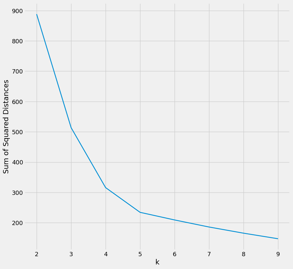 Figure 16: The plot generated from the elbow method suggests an optimal k value of 5.
Next, the KMeans algorithm is applied with k=5 to cluster the data based on the selected subset of columns. The clusters are then visualized in a 3D scatter plot, where each cluster is represented by a distinct color.
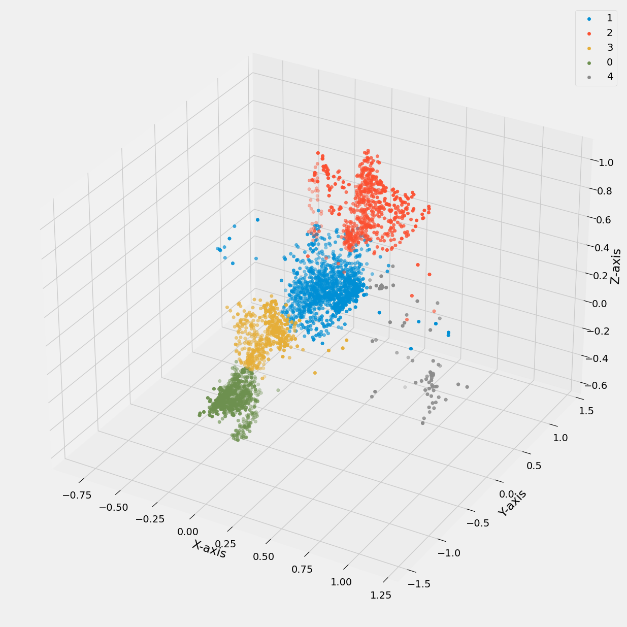 Figure 17: 3D scatter plot of accelerometer data vs cluster k value (0 to 4).
Additionally, its useful to compare the cluster plot to a plot of the original labels in the dataset.
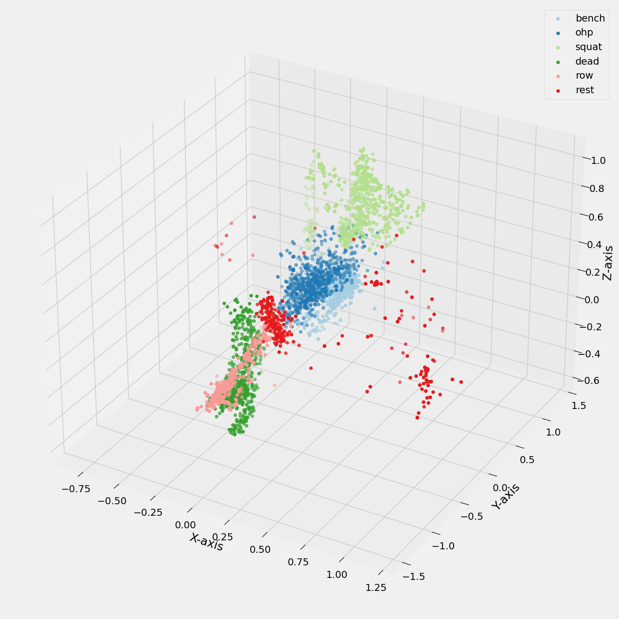 Figure 18: 3D scatter plot of accelerometer data vs Exercise Labels.
The figures depict 3D scatter plots illustrating the clustering of sensor data points based on exercise labels.
In Figure 17, distinct clusters are visible, indicating that the K-means model with five clusters has successfully separated the data points. However, upon closer inspection in Figure 18, it becomes evident that the clustering is not perfect, as certain exercises, such as overhead press and bench press, as well as deadlift and row, are not completely separated.
This overlap can be attributed to the similarities in motion patterns between these exercises, particularly in terms of movement along similar axes. Additionally, the spread of data points not belonging to any defined cluster in Figure 17 aligns with the variation observed during rest intervals between exercise sets, as shown in Figure 18.
Below, we present a similar comparison where the generated pca_1, pca_2, pca_3 values from our principal component analysis are utilized in conjunction with K-means to generate plots. In one plot, the legend corresponds to the k_number, while in another plot, it represents the exercise label.
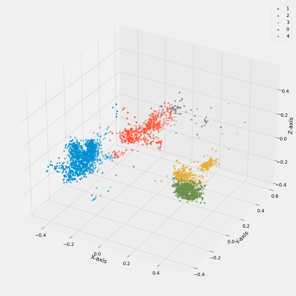 Figure 19: 3D scatter plot of pca data vs cluster k value (0 to 4).
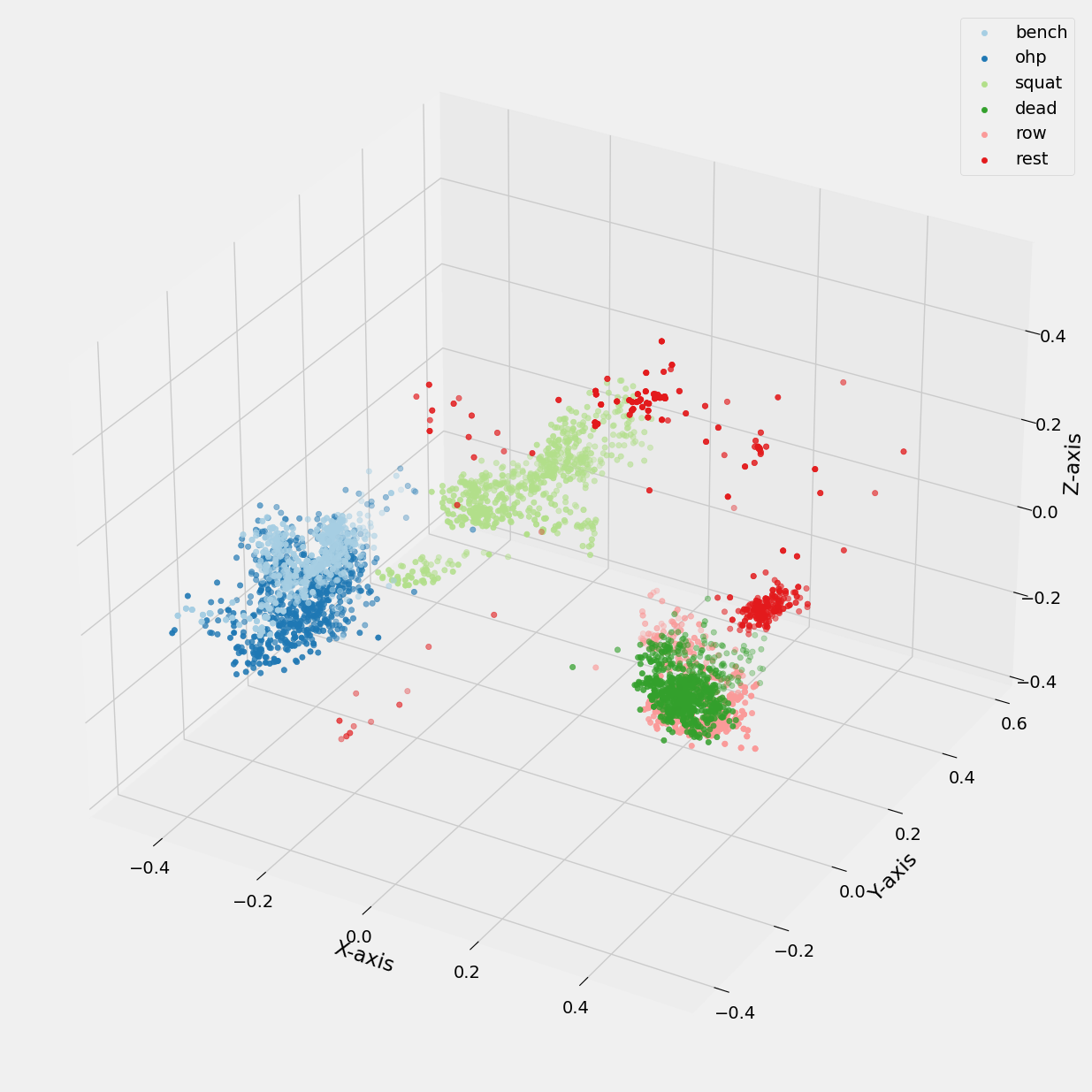 Figure 20: 3D scatter plot of pca values vs Exercise Labels.
Overall, while the clustering demonstrates some effectiveness in distinguishing between exercises, further refinement may be necessary to improve the model's accuracy and precision.
The final feature engineered datasaet is exported ready for further model development.
see file: data\interim\03_data_features.pkl
filepath : src\model\train_model.py
Exploration of feature selection, model selection, and hyperparameter tuning using grid search to identify the optimal combination leading to the highest classification accuracy.
Reading 03_data_features.pkl into a dataframe we then begin by creating a training and test sets using sklearn's train_test_split.
df_train = df.drop(["participant", "category", "set"], axis = 1)

X = df_train.drop("label", axis=1)
y = df_train["label"]

X_train, X_test, y_train, y_test = train_test_split(X, y, test_size=0.25, random_state=42, stratify=y)
Stratify parameter utilized for equal distribution of labels (Exercises).
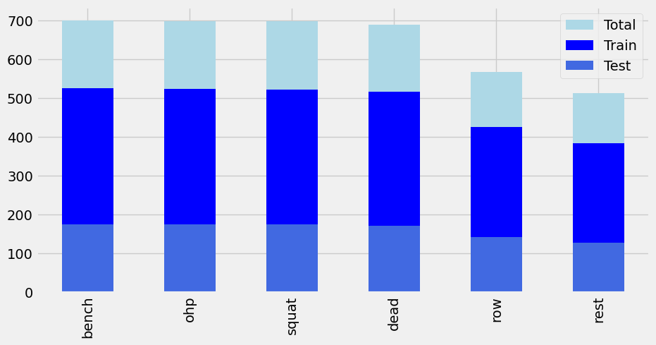 Figure 21: Distribution of data post Train-Test-Split with a test size of 25% of the total data.
Now we define our various feature sets which will be used to train and evaulate various models. testing models using a variety of different features will allow us to narrow down which features are most important for classification.
basic_features = ["acc_x","acc_y","acc_z","gyr_x","gyr_y","gyr_z"]
square_features = ["acc_r","gyr_r"]
pca_features = ["pca_1","pca_2","pca_3"]
time_features = [f for f in df_train.columns if "_temp_" in f]
frequency_features = [f for f in df_train.columns if ("_freq" in f) or ("_pse" in f)]
cluster_features = ["cluster"]

feature_set_1 = list(set(basic_features))
feature_set_2 = list(set(basic_features + square_features + pca_features))
feature_set_3 = list(set(feature_set_2 + time_features))
feature_set_4 = list(set(feature_set_3 + frequency_features + cluster_features))
We have a total of 116 features to consider.
basic_features: 6
square_features: 2
pca_features: 3
time_features: 16
frequency_features: 88
cluster_features: 1
Before utilizing the above features;
To give us some idea of what features could be most relevant, we implement forward selection, a method that iteratively selects the best features based on accuracy using a decision tree learner. We're looking for a maximum of 10 features.
Feedforward Neural Network: A powerful model for learning complex patterns in data, with options for hyperparameter tuning such as hidden layer sizes, activation functions, and learning rates.
learn = ClassificationAlgorithms()
max_features = 10

selected_features, ordered_features, ordered_scores = learn.forward_selection(max_features, X_train, y_train)
This approach helps reduce the dimensionality of the dataset and improve model performance by focusing on the most relevant features.
The forward selection returns the following 'selected_features':
selected_features = [
    'pca_1',
    'duration',
    'acc_z_freq_0.0_Hz_ws_14',
    'acc_y_temp_mean_ws_5',
    'acc_x_freq_1.071_Hz_ws_14',
    'gyr_x_freq_1.071_Hz_ws_14',
    'acc_z_freq_1.786_Hz_ws_14',
    'acc_x_freq_weighted',
    'acc_z_temp_std_ws_5',
    'acc_z_freq_weighted'
    ]
Resulting in our possible feature sets to test against looking like:
possible_feature_sets = [
    feature_set_1 ,
    feature_set_2 ,
    feature_set_3 ,
    feature_set_4 ,
    selected_features,
    ]
Using the LearningAlgorithms module we explore a variety of classification algorithms to build predictive models. For this project we use:
Feedforward Neural Network (NN): Employs multiple layers of nodes organized in a feedforward manner, allowing the network to learn complex patterns in the data by adjusting weights and biases during training.
k-Nearest Neighbors (kNN): A simple yet effective algorithm that classifies data points based on the majority class among their nearest neighbors. The number of neighbors (k) can be optimized using grid search.
Decision Tree (DT): An interpretable model that partitions the feature space based on simple decision rules. Parameters like the minimum samples per leaf and the splitting criterion can be tuned to improve model performance.
Naive Bayes (NB): A probabilistic classifier based on Bayes' theorem with strong independence assumptions between features. It is simple and fast, suitable for large datasets.
Random Forest (RF): An ensemble learning method that trains multiple decision trees and combines their predictions to improve generalization performance. Hyperparameters such as the number of trees and minimum samples per leaf can be optimized.
For each model, we utilize grid search to tune hyperparameters and identify the optimal combination leading to the highest classification accuracy.
Grid search exhaustively searches through a specified parameter grid to find the best parameters for each model. This process helps optimize model performance and generalization ability.
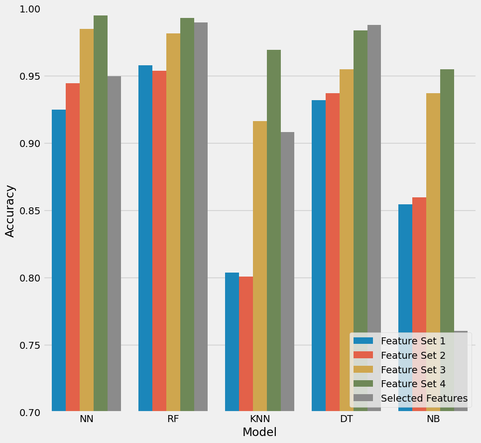 Figure 22: Visualisation of the accuracy of all models tested against the possible feature sets.
Referencing figure 22, we can observe how in almost all instances Feature_set_4 out perfoms all other features sets. NN and RF models seem to return the greatest accuracy for this feature set (>0.99).
Now its no real suprise that the best performing feature set is the one which contains all of the features however its interesting to learn that our best performing models are the Neural Network and the Random Forest models.
Evaluating the Neural Network model which used feature_set_4 returns a model with an accuracy of 0.994829 and the following confusion matrix:
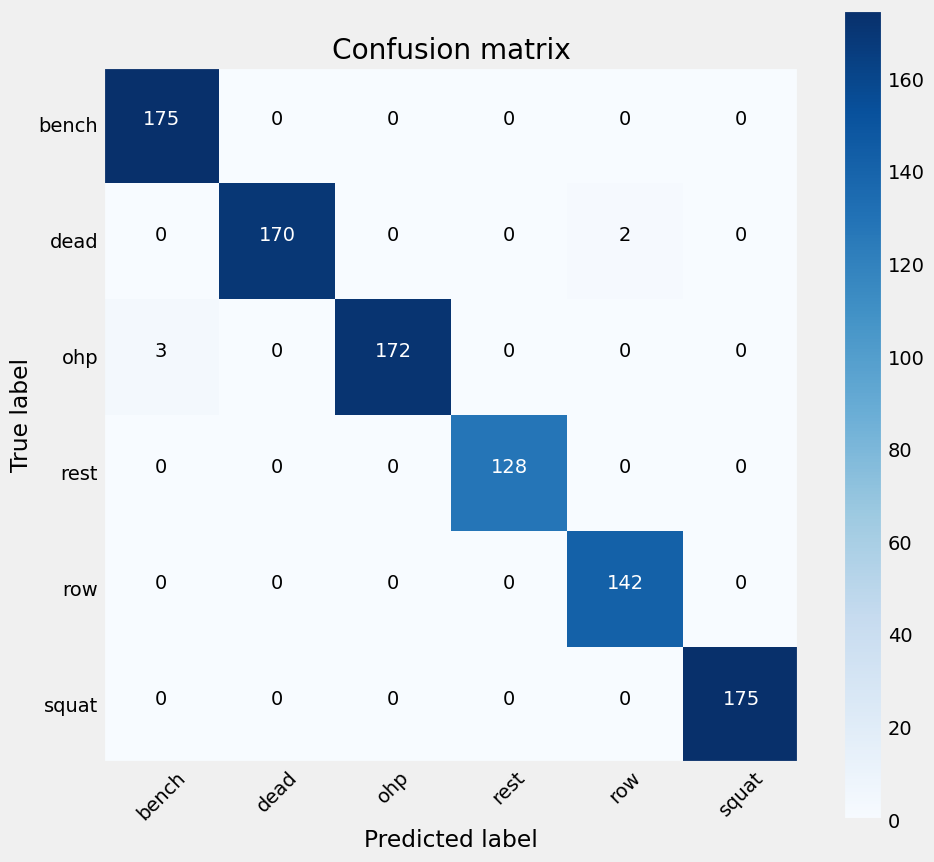 Figure 23: Confusion Matrix for the Neural Network model,showing a small discrepency in classifying OHP and deadlifts.
To evaluate the Neural Network model further, a new Train Test Split (TTS) was performed where we would exclude the data collected by Participant A from the training set but use only Participant A data in the testing sets.
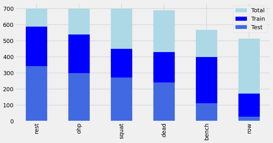 Figure 24: Distribution of data for Participant A Train Test Split
Evaluating the model again would return an accuracy of 0.992260 and the following confusion matrix:
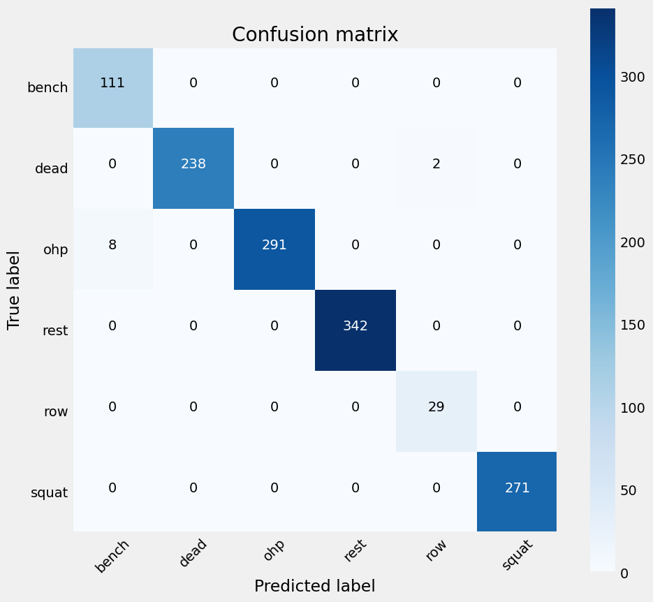 Figure 25: Confusion Matrix for the Neural Network model,showing an increased discrepency in classifying OHP and deadlifts when compared to Figure 23.
Furthermore the Random Forest model was evaluated using the same TTS as above, resulting in an accuracy score of 0.953560 and the following confusion matrix:
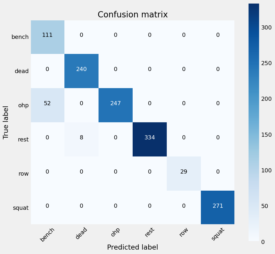 Figure 26: Confusion Matrix for the Random Forest model,showing a significantly increased discrepency in classifying OHP when compared to previous confusion matricies.
The accuracy is slightly reduced from the accuracy visualised in figure 22 due to the stochastic nature of the algorithm used.
Overall, the combination of feature selection, model selection, and hyperparameter tuning allows us to build robust predictive models for multiclass classification tasks, providing valuable insights into exercise/human activity recognition based on sensor data.