For this project, the Tennis environment was used.

In this environment, two agents control rackets to bounce a ball over a net. If an agent hits the ball over the net, it receives a reward of +0.1. If an agent lets a ball hit the ground or hits the ball out of bounds, it receives a reward of -0.01. Thus, the goal of each agent is to keep the ball in play.
The observation space consists of 8 variables corresponding to the position and velocity of the ball and racket. Each agent receives its own, local observation. Two continuous actions are available, corresponding to movement toward (or away from) the net, and jumping.
The task is episodic, and in order to solve the environment, your agents must get an average score of +0.5 (over 100 consecutive episodes, after taking the maximum over both agents). Specifically,
- After each episode, we add up the rewards that each agent received (without discounting), to get a score for each agent. This yields 2 (potentially different) scores. We then take the maximum of these 2 scores.
- This yields a single score for each episode.
The environment is considered solved, when the average (over 100 episodes) of those scores is at least +0.5.
Multi-Agent Deep Deterministic Policy Gradient (MADDPG) builds upon the Deep Deterministic Policy Gradient (DDPG) algorithm where multiple agents are coordinating to complete tasks with only local information. In the viewpoint of one agent, the environment is non-stationary as policies of other agents are quickly upgraded and remain unknown. MADDPG is an actor-critic model redesigned particularly for handling such a changing environment and interactions between agents.
More concretely, consider a game with N agents with policies parameterized by θ = {θ1, ..., θN }, and let π = {π1, ..., πN } be the set of all agent policies. Then we can write the gradient of the expected return for agent i, J(θi) = E[Ri] as:

Here Qiπ(x, a1, ..., aN ) is a centralized action-value function that takes as input the actions of all agents, a1, . . . , aN , in addition to some state information x, and outputs the Q-value for agent i. In the simplest case, x could consist of the observations of all agents, x = (o1, ..., oN ), however we could also include additional state information if available. Since each Qiπ is learned separately, agents can have arbitrary reward structures, including conflicting rewards in a competitive setting.
We can extend the above idea to work with deterministic policies. If we now consider N continuous policies µθi w.r.t. parameters θi (abbreviated as µi), the gradient can be written as: ∇θiJ(µi) = Ex,a∼D[∇θiµi(ai|oi)∇aiQ µ i (x, a1, ..., aN )|ai=µi(oi)],
The problem can be formalized in the multi-agent version of MDP, also known as Markov games. Say, there are N agents in total with a set of states S. Each agent owns a set of possible action, A1,…,AN, and a set of observation, O1,…,ON. The state transition function involves all states, action and observation spaces T : S×A1×…AN ↦ S. Each agent’s stochastic policy only involves its own state and action: πθi : Oi×Ai ↦ [0,1], a probability distribution over actions given its own observation, or a deterministic policy: μθi : Oi ↦ Ai.
Let o =o1,…,oN, μ =μ1,…,μN and the policies are parameterized by θ =θ1,…,θN.
The critic in MADDPG learns a centralized action-value function Qiμ(o ,a1,…,aN) for the i-th agent, where a1∈A1,…,aN∈AN are actions of all agents. Each Qiμ i is learned separately for i=1,…,N and therefore multiple agents can have arbitrary reward structures, including conflicting rewards in a competitive setting. Meanwhile, multiple actors, one for each agent, are exploring and upgrading the policy parameters θ1 on their own.
Actor update:

Where D is the memory buffer for experience replay, containing multiple episode samples (o , a1,…,a N, r1,…,rN, o′ ) — given current observation o , agents take action a1,…,aN and get rewards r1,…,rN, leading to the new observation o ′.
Critic update:
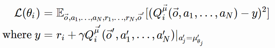
where μ′ are the target policies with delayed softly-updated parameters.
If the policies μ are unknown during the critic update, we can ask each agent to learn and evolve its own approximation of others’ policies. Using the approximated policies, MADDPG still can learn efficiently although the inferred policies might not be accurate.
To mitigate the high variance triggered by the interaction between competing or collaborating agents in the environment, MADDPG proposed one more element - policy ensembles:
- Train K policies for one agent;
- Pick a random policy for episode rollouts;
- Take an ensemble of these K policies to do gradient update.
In summary, MADDPG added three additional ingredients on top of DDPG to make it adapt to the multi-agent environment:
- Centralized critic + decentralized actors;
- Actors are able to use estimated policies of other agents for learning;
- Policy ensembling is good for reducing variance.
Below, the pseudocode is described:

The next two entries visualize the flow diagrams for the Network. This work builds upon implementations from the first DRLND project Navigation and the second DRLND project Continuous Control.
Below, the flow diagram demonstrates how the Actor network is setup.
model = Actor(state_size, action_size, 42)
model.eval()
x = Variable(torch.randn(1,state_size))
y = model(x)

make_dot(y, params=dict(list(model.named_parameters())))
Below, the flow diagram demonstrates how the Critic network is setup.
model = Critic(state_size, action_size, 42)
model.eval()
x = Variable(torch.randn(1,state_size))
z = Variable(torch.randn(1,action_size))
y = model(x, z)

make_dot(y, params=dict(list(model.named_parameters())))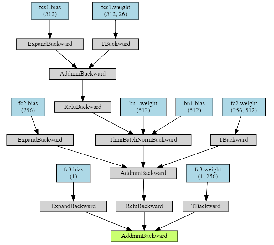
Note: the original OpenAI MADDPG implementation for policy ensemble and policy estimation can be found here. The code is provided as-is.
NB: Code will run in GPU if CUDA is available, otherwise it will run in CPU.
Code is structured in different modules. The most relevant features will be explained next:
- model.py: It contains the main execution thread of the program. This file is where the main algorithm is coded (see algorithm above). PyTorch is utilized for training the agent in the environment. The agent has an Actor and Critic network.
- ddpg_agent.py: The model script contains the DDPG agent, a Replay Buffer memory, and the Q-Targets feature.
- maddpg_agent.py: Augments the DDPG
learn()function for MADDPG via amaddpg_learn()method using batches to handle the value parameters and update the policy forQ_targets. - hyperparameters.py: Allows for a common module to inherit preset hyperparameters for all modules.
- memory.py: Instantiates the buffer replay memory module.
- Tennis.ipynb: The Navigation Jupyter Notebook provides an environment to run the Tennis game, import dependencies, train the MADDPG, visualize via Unity, and plot the results.
The PyTorch saved model can be loaded with ac = torch.load('path/to/model.pt'), yielding an actor-critic object (ac) that has the properties described in the docstring for ddpg_pytorch.
You can get actions from this model with:
actions = ac.act(torch.as_tensor(obs, dtype=torch.float32))The DDPG agent uses the following parameters values (defined in parameters.py)
SEED = 10                           # Random seed
NB_EPISODES = 10000                 # Max nb of episodes
NB_STEPS = 1000                     # Max nb of steps per episodes
UPDATE_EVERY_NB_EPISODE = 4         # Nb of episodes between learning process
MULTIPLE_LEARN_PER_UPDATE = 3       # Nb of multiple learning process performed in a row

BUFFER_SIZE = int(1e5)              # Replay buffer size
BATCH_SIZE = 256                    # Batch size #128
ACTOR_FC1_UNITS = 512               # Number of units for L1 in the actor model #256
ACTOR_FC2_UNITS = 256               # Number of units for L2 in the actor model #128
CRITIC_FCS1_UNITS = 512             # Number of units for L1 in the critic model #256
CRITIC_FC2_UNITS = 256              # Number of units for L2 in the critic model #128
NON_LIN = F.relu                    # Non linearity operator used in the model #F.leaky_relu
LR_ACTOR = 1e-4                     # Learning rate of the actor #1e-4
LR_CRITIC = 5e-3                    # Learning rate of the critic #1e-3
WEIGHT_DECAY = 0                    # L2 weight decay #0.0001

GAMMA = 0.995                       # Discount factor #0.99
TAU = 1e-3                          # For soft update of target parameters
CLIP_CRITIC_GRADIENT = False        # Clip gradient during Critic optimization

ADD_OU_NOISE = True                 # Toggle Ornstein-Uhlenbeck noisy relaxation process
THETA = 0.15                        # k/gamma -> spring constant/friction coefficient [Ornstein-Uhlenbeck]
MU = 0.                             # x_0 -> spring length at rest [Ornstein-Uhlenbeck]
SIGMA = 0.2                         # root(2k_B*T/gamma) -> Stokes-Einstein for effective diffision [Ornstein-Uhlenbeck]
NOISE = 1.0                         # Initial Noise Amplitude
NOISE_REDUCTION = 0.995             # Noise amplitude decay ratio
With the afformentioned setup, the agent was able to successfully meet the functional specifications in 3193 episodes with an average score of [0.50 2.60] (see below):
Episode 100     Average Score: 0.00 (nb of total steps=1466     noise=0.0006)
Episode 200     Average Score: 0.01 (nb of total steps=3066     noise=0.0000)
Episode 300     Average Score: 0.03 (nb of total steps=5204     noise=0.0000)
Episode 400     Average Score: 0.01 (nb of total steps=6840     noise=0.0000)
Episode 500     Average Score: 0.00 (nb of total steps=8291     noise=0.0000)
Episode 600     Average Score: 0.00 (nb of total steps=9711     noise=0.0000)
Episode 700     Average Score: 0.00 (nb of total steps=11131    noise=0.0000)
Episode 800     Average Score: 0.01 (nb of total steps=12726    noise=0.0000)
Episode 900     Average Score: 0.05 (nb of total steps=15057    noise=0.0000)
Episode 1000    Average Score: 0.02 (nb of total steps=17013    noise=0.0000)
Episode 1100    Average Score: 0.06 (nb of total steps=19768    noise=0.0000)
Episode 1200    Average Score: 0.05 (nb of total steps=22160    noise=0.0000)
Episode 1300    Average Score: 0.05 (nb of total steps=24842    noise=0.0000)
Episode 1400    Average Score: 0.05 (nb of total steps=27546    noise=0.0000)
Episode 1500    Average Score: 0.05 (nb of total steps=30057    noise=0.0000)
Episode 1600    Average Score: 0.05 (nb of total steps=32885    noise=0.0000)
Episode 1700    Average Score: 0.05 (nb of total steps=35902    noise=0.0000)
Episode 1800    Average Score: 0.06 (nb of total steps=39120    noise=0.0000)
Episode 1900    Average Score: 0.10 (nb of total steps=43527    noise=0.0000)
Episode 2000    Average Score: 0.06 (nb of total steps=46890    noise=0.0000)
Episode 2100    Average Score: 0.08 (nb of total steps=50792    noise=0.0000)
Episode 2200    Average Score: 0.07 (nb of total steps=54382    noise=0.0000)
Episode 2300    Average Score: 0.08 (nb of total steps=58002    noise=0.0000)
Episode 2400    Average Score: 0.11 (nb of total steps=62226    noise=0.0000)
Episode 2500    Average Score: 0.06 (nb of total steps=64770    noise=0.0000)
Episode 2600    Average Score: 0.05 (nb of total steps=67201    noise=0.0000)
Episode 2700    Average Score: 0.09 (nb of total steps=71145    noise=0.0000)
Episode 2800    Average Score: 0.12 (nb of total steps=75897    noise=0.0000)
Episode 2900    Average Score: 0.13 (nb of total steps=81294    noise=0.0000)
Episode 3000    Average Score: 0.22 (nb of total steps=89657    noise=0.0000)
Episode 3100    Average Score: 0.41 (nb of total steps=105475   noise=0.0000)
Environment solved in 3193 episodes with an Average Score of 0.50 2.60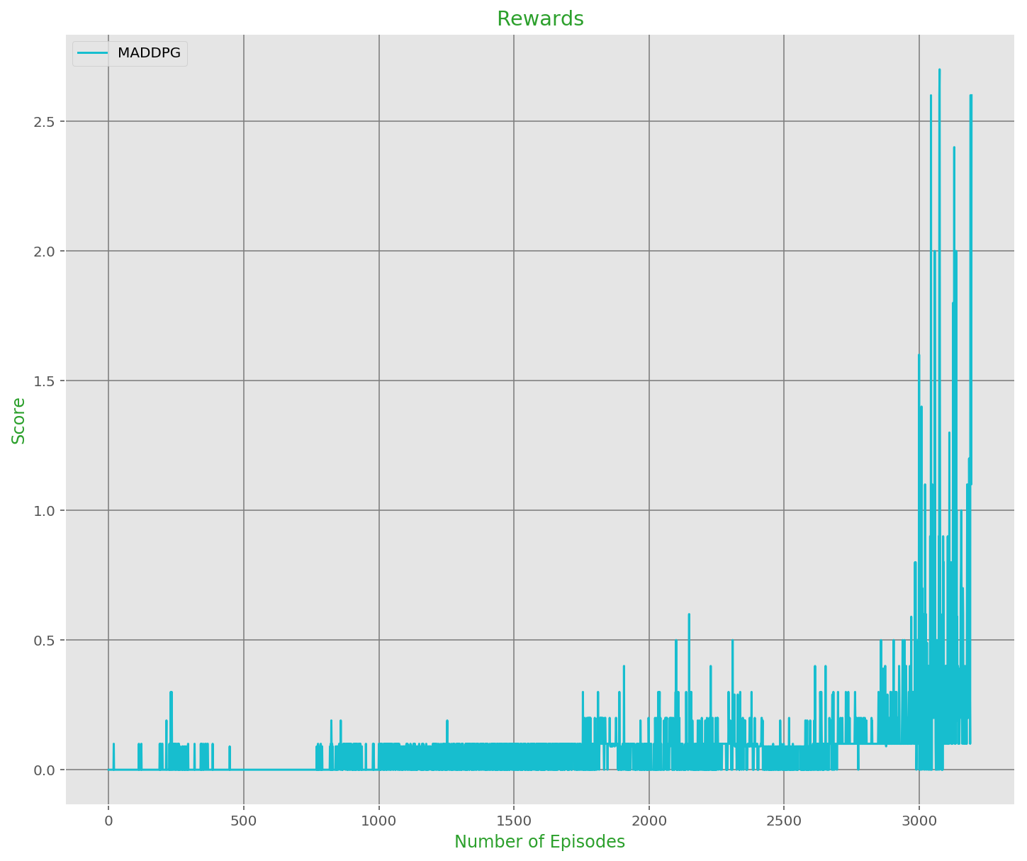
This section contains two additional algorithms that would vastly improve over the current implementation, namely TRPO and TD3. Such algorithms have been developed to improve over DQNs and DDPGs.
We describe an iterative procedure for optimizing policies, with guaranteed monotonic improvement. By making several approximations to the theoretically-justified procedure, we develop a practical algorithm, called Trust Region Policy Optimization (TRPO). This algorithm is similar to natural policy gradient methods and is effective for optimizing large nonlinear policies such as neural networks. Our experiments demonstrate its robust performance on a wide variety of tasks: learning simulated robotic swimming, hopping, and walking gaits; and playing Atari games using images of the screen as input. Despite its approximations that deviate from the theory, TRPO tends to give monotonic improvement, with little tuning of hyperparameters.
Twin Delayed Deep Deterministic policy gradient algorithm (TD3), an actor-critic algorithm which considers the interplay between function approximation error in both policy and value updates. We evaluate our algorithm on seven continuous control domains from OpenAI gym (Brockman et al., 2016), where we outperform the state of the art by a wide margin. TD3 greatly improves both the learning speed and performance of DDPG in a number of challenging tasks in the continuous control setting. Our algorithm exceeds the performance of numerous state of the art algorithms. As our modifications are simple to implement, they can be easily added to any other actor-critic algorithm.
Further more, the Crawler environment will be explored at a later time.

[1] Mordatch et al. (OpenAI), Emergence of Grounded Compositional Language in Multi-Agent Populations.
[2] Lowe et al. (OpenAI), Multi-Agent Actor-Critic for Mixed Cooperative-Competitive Environments.