Audio Processing Tutorial Book

---

>> Tools used:

---

>> Installing tools:

---

1. python

Python 3.7.15

2. pydub

 pip install pydub==0.25.1 

3. librosa

pip install librosa==0.8.1

4. numpy

pip install numpy==1.21.6

5. matplotlib

pip install matplotlib==3.2.2

1. >>> Reading Audio file

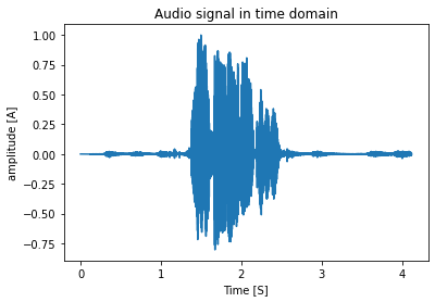
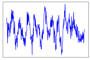
• We read audio files using librosa python package. Librosa is a tool used for music and audio analysis and processing.

• its a 4 second audio with sample rate : 22050 samples / second.

• sample plot of the audio signal is given below:

• the original audio is displayed below:

1.org.mov

2. >>> Voice Activity Detection (VAT) and audio clipping.

• Voice activity detection (VAD) is a technique in which the presence or absence of human speech is detected.
• We begin by normalising the audio signal so that its amplitude falls between -1 and +1.
• Next, we assign a threshold value above which when the signal goes, it will be a speech signal and all other below are noises and thus not considered.
• Through this process, we select our area of interest from the audio sample, and from that index range, we clip the audio and generate the desired output.
• sample plot of the audio signal after VAD and clipping is given below:

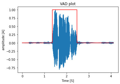
• the red graph is the VAD plot and the blue one is the audio signal.
• The area where the red pulse occured is our area of interest.
• after selecting the range we will clip the audio sample in that selected range, a cropped audio signal plot is given below:
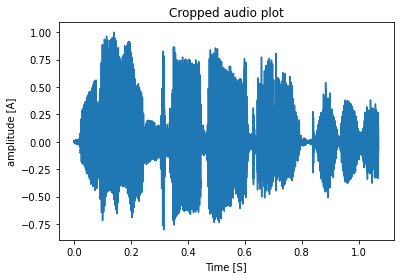
• so after cropping the audio only contains speech / human voice the silent part gets removed and thus the duration also gets reduced.
• the cropped audio / audio after clipping is displayed below:

2.vad_croped.mov

3. >>> Pre-Emphasis

• The first step is to apply a pre-emphasis filter on the signal to amplify the high frequencies. A pre-emphasis filter is useful in several ways: (1) balance the frequency spectrum since high frequencies usually have smaller magnitudes compared to lower frequencies, (2) avoid numerical problems during the Fourier transform operation and (3) may also improve the Signal-to-Noise Ratio (SNR).

The pre-emphasis filter can be applied to a signal x using the first order filter in the following equation:

$y(t)=x(t)−αx(t−1)$

• where α is the filter coefficient we take its value as 0.97 in most of the cases.
• sample plot of the audio signal after pre-emphasis is given below:

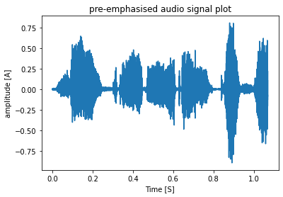
• pre-emphasised audio is displayed below:

3.preempha.mov

4. >>> sampling audio signal

• first of all we are splitting the audio signal or applying a sliding window to the audio signal so that we will get n- number of audio samples of equal time duration / intervals (we are taking 10ms audio samples).

• full audio signal as continuous plots of 10ms samples is given below:

• a single audio sample will looks like this:

5. >>> applying hann-window function to each audio samples

• We use the hann-window function to limit spectrum leakage, smooth the beginning and end of each audio sample we previously prepared, and challenge the FFT's assumption that the data is endless.
• The following equation generates the coefficients of a Hann window:

$w(n)=0.5(1−cos(2πnN)),0≤n≤N$

The window length $L = N + 1$.

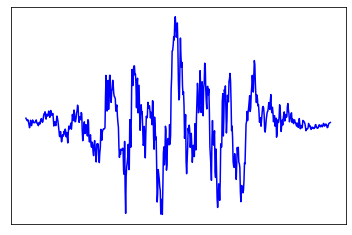
• full audio signal as continuous plots of 10ms samples after applying hann-window function is given below:

• a single audio sample after applying hann-window function will looks like this:

• audio signal after applying window function is dispalyed below:

5.hann_windowed.mov

6. >>> time domain to frequency domain conversion of audio signal

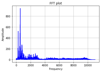
• we use Fast Fourier Transform (FFT) to do this conversion task.

• after this conversion a signal in time domain will be converted to frequency domain.

• audio signal in time domain ( X-axis time ) is shown below:

• Audio signal after applying FFT , now in frequency domain (X-axis frequency) is shown below:

7. >>> spectrogram of the audio signal

• A spectrogram is a visual representation of the spectrum of frequencies of a signal as it varies with time. It’s a representation of frequencies changing with respect to time for given audio signals.

• In spectrogram we have time in X-axis and frequency in Y-axis.

• audio signal spectrogram is shown below:

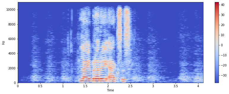
• The colour intensity shows the variation in power level of audio signal in (dB), red colour indicates more power and blue indicates low power areas.

8. >>> MFCC ( Mel-frequency Cepstral Coefficients ) feature extraction

• mel-scale comes from the fact that human ear is highly sensitive to small changes made in the low frequency components. mel-scale is almost linear for frequency below 1000 Hz, and logarithmic for frequency above 1000 Hz, thus following the same pattern as that of the human ear.

• The mel frequency cepstral coefficients (MFCCs) of a signal are a small set of features (usually about 10-20) which concisely describe the overall shape of a spectral envelope.

• MFCC features are widely used in speech recognition problems. Speech is dictated by the way in which we use our oral anatomy to create each sound. Therefore, one way to uniquely identify a sound (independent of the speaker) is to create a mathematical representation that encodes the physical mechanics of spoken language. MFCC features are one approach to encoding this information.

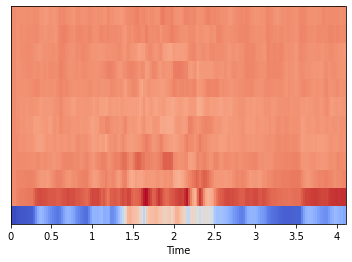
• In MFCC plot we have time in X-axis and n number of MFCC features in Y-axis in our case it is 12 only.

• MFCC feature plot is shown below:

9. >>> Reconstruction of audio from MFCC features

• We can rebuild our original signal from MFCCs up to a certain degree even if they are a very compressed version of our original audio signal; nonetheless, acceptable losses must be taken into account.
• a reconstructed version of above audio signal is displayed below:

4.reconstructed.mov

THE END

---