TreeProfiler is a command line tool designed to automate the annotation of large phylogenetic trees with corresponding metadata. It also facilitates the visual exploration of these annotations as phylogenetic profiles, making it a powerful resource for researchers working with complex biological data.
Key Features:
- Automated Annotation that integrates metadata into phylogenetic tree, and summarizes annotation in internal nodes, including:
- Categorical/Numerical metadata in TSV/CSV format
- Taxonomic Annotation of NCBI/GTDB taxonomy database
- Functional Annotation from eggnog-mapper output
- Domain annotation from pfam/smart
- Multiple Sequence Alignment annotation
- Visual Exploration that allows for the detailed examination of annotated trees, aiding in the interpretation and presentation of data.
- Analytic Methods for computing analysis from leaf nodes:
- Ancestral Character Reconstruction for both discrete and continuous traits.
- Phylogenetic Signal Delta Statistic]
- Lineage Specificity Analysis
The official documentation of TreeProfiler is in https://dengzq1234.github.io/TreeProfiler/ where provides detailed instructions with examples.
If you have any doubts, please drop a line in issue or contact https://x.com/deng_ziqi
Full manuscript of TreeProfiler is in https://doi.org/10.1101/2023.09.21.558621
If you use TreeProfiler, please cite:
Ziqi Deng, Ana Hernández-Plaza, Jaime Huerta-Cepas.
"TreeProfiler: A command-line tool for computing and visualizing phylogenetic profiles against large trees"
bioRxiv (2023) doi: 10.1101/2023.09.21.558621
-
- Parsing Input tree
- treeprofiler-annotate, computing phylogenetic profiles and annotation
- treeprofiler-plot visualizing phylogenetic profiles and annotation
- Interactive visualization interface
- Basic options of visualizing layouts
- Layouts for categorical data
- Layouts for boolean data
- Layouts for numerical data
- Layouts for Analytical Data
- Layouts for multiple sequence alignment
- Layouts for eggnog-mapper pfam annotations
- Layouts for eggnog-mapper smart annotations
- Layouts for eggnog-mapper annotations
- Layouts for Taxonomic data
- Customize color in layout with color config
- Conditional query in annotated tree
-
Demo1 Explore GTDB taxonomic tree with metadata and habitat information of progenome3
TreeProfiler is command-line tool for profiling metadata table into phylogenetic tree with descriptive analysis and output visualization
TreeProfiler requires
- Python version >= 3.10
- ETE Toolkit v4
- biopython >= 1.8
- selenium >= 4.24
- scipy >= 1.8.0
- matplotlib >= 3.4
- pymc >= 5.0.0
- numpy == 1.24.4
- aesara
- pastml (custom)
- webdriver_manager
- pyvirtualdisplay
# Install ETE Toolkit v4
pip install --force-reinstall https://github.com/etetoolkit/ete/archive/ete4.zip

# Install custom pastml package for ete4
pip install "git+https://github.com/dengzq1234/pastml.git@pastml2ete4"

# Install TreeProfiler tool via pip
pip install TreeProfiler

# Or install directly from github
pip install https://github.com/compgenomicslab/TreeProfiler/archive/main.zip
# or development mode for latestest update
pip install git+https://github.com/compgenomicslab/TreeProfiler@dev-repo
TreeProfiler provide various example dataset for testing in examples/ or https://github.com/compgenomicslab/TreeProfiler/tree/main/examples,
each directory consists a demo script *_demo.sh for quick starting different functions in TreeProfiler which alreadyh as annotate-plot pipeline of example data. User can fast explore different example tree with different visualizations. Here is the demonstration:
# execute demo script of example1
cd examples/basic_example1/
sh ./example1_demo.sh

Annotate example tree with two metadata tables
start parsing...
Time for parse_csv to run:  0.001968860626220703
Time for load_metadata_to_tree to run:  0.0003094673156738281
Time for merge annotations to run:  0.05160331726074219
Time for annotate_taxa to run:  4.76837158203125e-07
Visualize properties categorical data random_type in rectangle_layout, numerical data sample1, sample2 in heatmap_layout and barplot_layout.
Current trees in memory: 0
Added tree example with id 0.
 * Serving Flask app 'ete4.smartview.gui.server' (lazy loading)
 * Environment: production
   WARNING: This is a development server. Do not use it in a production deployment.
   Use a production WSGI server instead.
 * Debug mode: on
 * Running on http://127.0.0.1:5000/ (Press CTRL+C to quit)
As the session starts in local server http://127.0.0.1:5000, annotated tree and selected properties are visualized at the interactive session.
 Here is detailed introduction of interactive session of visualization(here)
Check other tutorial scripts
# display demo script of each example
./examples/basic_example1/example1_demo.sh
./examples/automatic_query/highlight_demo.sh
./examples/automatic_query/collapse_demo.sh
./examples/automatic_query/prune_demo.sh
./examples/basic_example2/example2_demo.sh
./examples/taxonomy_example/ncbi/ncbi_demo.sh
./examples/taxonomy_example/gtdb/gtdb_demo.sh
./examples/pratical_example/progenome3/progenome_demo.sh
./examples/pratical_example/gtdb_r202/gtdbv202full_demo.sh
./examples/pratical_example/gtdb_r202/gtdbv202lite_demo.sh
./examples/pratical_example/emapper/emapper_demo.sh
Quick way
pip install https://github.com/etetoolkit/ete/archive/ete4.zip
For local development To install ETE in a local directory to help with the development, you can:
- Clone this repository (git clone https://github.com/etetoolkit/ete.git)
- Install dependecies
- If you are using conda:
conda install -c conda-forge cython bottle brotli pyqt numpy<2.0 - Otherwise, you can install them with
pip install <dependencies> - Build and install ete4 from the repository's root directory:
pip install -e .
- If you are using conda:
(In Linux there may be some cases where the gcc library must be installed, which can be done with conda install -c conda-forge gcc_linux-64)
Install dependencies
# install BioPython, selenium, scipy via conda
conda install -c conda-forge biopython selenium scipy matplotlib pymc aesara
# or pip
pip install biopython selenium scipy matplotlib pymc aesara webdriver_manager pyvirtualdisplay
Install TreeProfiler
# install TreeProfiler
git clone https://github.com/compgenomicslab/TreeProfiler
cd TreeProfiler/
python setup.py install
Or
# install directly
pip install https://github.com/compgenomicslab/TreeProfiler/archive/main.zip
TreeProfiler takes following file types as input
| Input | Filetype |
|---|---|
| Tree | newick, ete |
| Metadata | tar.gz, tsv |
- ete format is a novel format developed to solve the situation we encounter in the previous step, annotated tree can be recover easily with all the annotated data without changing the data type. Besides, the ete format optimized the tree file size after mapped with its associated data. Hence it's very handy for programers in their own script. At this moment we can only view the ete format in treeprofiler, but we will make the ete format more universal to other phylogenetic software.
- Metadata input could be single or multiple files, either tar.gz compressed file(s) which contains multiple .tsv or plain .tsv file(s).
TreeProfiler has two main subcommand:
- annotate
- plot
The first one annotate is used to annotate your input tree and corresponding metadata, TreeProfiler will map all the metadata into corresponding tree node. In this step, annotated tree will be generated in newick and ete format
treeprofiler annotate --tree tree.nw --input-type newick --metadata metadata.tsv --outdir ./
The second subcommand plot is used to visualize tree with associated metadata. By default, treeprofiler will launch an interactive session at localhost for user to explore input tree.
treeprofiler plot --tree tree_annotated.nw --input-type newick
or
treeprofiler plot --tree tree_annotated.ete --input-type ete
In this Tutorial we will use TreeProfiler and demostrate basic usage with data in examples/
TreeProfiler accpept input tree in .nw or .ete by putting --input-type {newick,ete} flag to identify. By default, TreeProfiler will automatically detech the format of tree. The difference between .nw and .ete:
-
newickformat is more universal and be able to used in different other phylogenetic software although associated data of tree nodes will be considered as plain text. -
eteformat is a novel format developed to solve the situation we encounter in the previous step, annotated tree can be recover easily with all the annotated data without changing the data type. Besides, the ete format optimized the tree file size after mapped with its associated data. Hence it's very handy for programers in their own script. At this moment we can only view the ete format in treeprofiler, but we will make the ete format more universal to other phylogenetic software. Hence using ete format inplotsubcommand is highly reccomended
TreeProfiler provides argument --internal {name,support} to specify newick tree when it include values in internal node. [default: name]
| newick | leaves | internal_node value | internal_parser |
|---|---|---|---|
| (A:0.5, B:0.5)Internal_C:0.5; | A, B | Internal_C | name |
| (A:0.5, B:0.5)0.99:0.5; | A, B | 0.99 | support |
TreeProfiler annotate subcommand is the step that annotate input metadata to target tree. As a result, itwill generate the following output file:
<input_tree>+ _annotated.nw, newick format with annotated tree<input_tree>+ _annotated.ete, ete format with annotated tree<input_tree>+ _annotated_prop2type.txt, config file where store the datatype of each annotated properties<input_tree>+ _annotated.tsv, metadata in tab-separated values format with annotated and summarized internal nodes information.
In the following sub session we will describe the usage of following arguments in annotate step for metadata:
| Argument | Description |
|---|---|
-d, --metadata METADATA [METADATA ...] |
<metadata.csv> .csv, .tsv filename |
-s, --metadata-sep METADATA_SEP |
Column separator of metadata table [default: \t] |
--data-matrix DATA_MATRIX [DATA_MATRIX ...] |
<datamatrix.csv> .csv, .tsv. Numerical matrix data metadata table as array to tree, please do not provide column headers in this file, filename will become the property name in the tree. |
--no-headers |
Metadata table doesn't contain columns name, namespace col+index will be assigned as the key of property such as col1. |
--duplicate |
Treeprofiler will aggregate duplicated metadata to a list as a property if metadata contains duplicated row. |
TreeProfiler allows users to input metadata in tsv/csv file by setting --metadata <filename.tsv|.csv> and -s <seperator>. By default, the first column of metadata should be names of target tree leaves and metadata should contain column names for each column of metadata.
TreeProfiler allows user to annotate more than one metadata inputs to tree such as --metadata table1.tsv table2.tsv.
Check metadata
cd examples/basic_example0/
tree ./
./
├── boolean.tsv
├── categorical_duplicated.tsv
├── categorical.tsv
├── data.array
├── demo1.tree
├── numerical.tsv
└── show_tree_props.py

# check metadata structure
head categorical.tsv
name,categorical1
Taxa_0,A
Taxa_1,B
Taxa_2,B
Taxa_3,C
Run annotate subcommand
## annotate tree with more than one metadata tsv, seperated by `,`
# set the correct filename and seperator
treeprofiler annotate \
-t demo1.tree \
--metadata categorical.tsv \
-sep , \
-o .
After annotation, treeprofiler will generate annotated tree
ls demo1*
demo1_annotated.ete  demo1_annotated.nw  demo1_annotated.tsv  demo1_prop2type.txt  demo1.tree
Now we can check annotated tree
# show tree's properties
python show_tree_props.py demo1_annotated.nw

Target tree internal node Root contains the following properties:
{'categorical1_counter': 'A--1||B--2||C--2', 'name': 'Root'}
Target tree leaf node Taxa_0 contains the following propertiies:
{'name': 'Taxa_0', 'dist': 0.190563, 'categorical1': 'A'}
treeprofiler can handle the whole tsv/csv file as one property and annotate it to related leaves, by using --data-matrix <filename.tsv|.csv> It must be numerical data matrix and without headers. Once annotated the property of data-matrix will be named by the filename (see example below)
The difference between --data-matrix and --metadata is that the former sees the whole metadata file as a node property and stores the rows as an array in leaf nodes, and the latter sees each column from metadata as each single property of leaf nodes.
Using data array file data.array from the previous example
# annotated data.array file to tree
treeprofiler annotate \
-t demo1.tree \
--data-matrix data.array \
-sep , \
-o .

# data.array is stored as one property in tree node and value is stored as array
python show_tree_props.py demo1_annotated.nw
target tree internal node Root contains the following properties:
{
'data.array_avg': '1.0244|-0.667|-1.7740000000000002|-0.8620000000000001|-0.6552',
'data.array_max': '3.671|1.937|4.362|1.585|2.746',
'data.array_min': '-2.591|-2.356|-4.825|-3.326|-2.479',
'data.array_std': '2.3121192529798287|1.5156064132880938|3.524138873540599|1.9937640783202009|1.906460531980665',
'data.array_sum': '5.122|-3.335|-8.870000000000001|-4.3100000000000005|-3.276',
'name': 'Root'
}
target tree leaf node Taxa_0 contains the following propertiies:
{
'name': 'Taxa_0',
'dist': 0.190563,
'data.array': '-2.591|1.937|-3.898|0.447|-1.349'
}
If metadata doesn’t have headers, by setting --no-headers to set the metadata properly, therefore treeprofiler will name each column by col+<column number> as the property key in each leaf node, such as col1, col2, etc.
example
# data.array doesn't have headers for each column
head data.array
Taxa_0,-2.591,1.937,-3.898,0.447,-1.349
Taxa_1,3.366,-1.871,4.362,1.585,-2.479
Taxa_2,0,-0.098,0,-3.326,2.746
Taxa_3,3.671,-0.947,-4.509,-3.131,-2.194

# need to add --no-headers flag to tell treeprofiler
treeprofiler annotate \
-t demo1.tree \
--metadata data.array \
-sep , \
--no-headers \
-o .

# check properties
python show_tree_props.py demo1_annotated.nw
target tree internal node Root contains the following properties:
{'col1_avg': '1.92825',
'col1_max': '3.671',
'col1_min': '0.0',
'col1_std': '3.463526916666666',
'col1_sum': '7.713',
'col2_avg': '-1.318',
...}

target tree leaf node Taxa_0 contains the following propertiies:
{'name': 'Taxa_0',
'dist': 0.190563,
'col1': '-2.591',
'col2': '1.937',
'col3': '-3.898',
'col4': '0.447',
'col5': '-1.349'}
Metadata column which fullfills one of the following criterias will be consider as missing value:
- Entirely symbolic characters. Such as
+,-,~,., etc. - The exact strings
none,None,null,Null, orNaN. - An empty string (zero characters).
Missing value will replaced by string 'NaN' in the corresponding property.
If Metadata doesn't cover input tree leaf, tree leaf will be unannotated.
In general, treeprofiler expects each row of metadata corresponding to one leaf, such as
head categorical.tsv
#name,categorical1
Taxa_0,A
Taxa_1,B
Taxa_2,B
Taxa_3,C
Taxa_4,C
Although treeprofiler can handle metadata with rows with duplicated leafnames such as
head categorical_duplicated.tsv
#name,categorical1
Taxa_0,A
Taxa_0,B
Taxa_2,B
Taxa_2,C
Taxa_3,C
Taxa_3,A
Taxa_4,C
In order to do so, users need to add --duplicate , by doing so, metadata from the same leaf will be aggregate into the same column. Such as the Taxa_0 from the above table, at the end value A and B will be both annotated to property categorical1(see above demo). If not, treeprofielr will take one the first row of metadata that appear as the metadata for related leaf!
example
treeprofiler annotate \
-t demo1.tree \
-d categorical_duplicated.tsv \
-sep , \
--duplicate \
-o .

python show_tree_props.py demo1_annotated.nw
target tree internal node Root contains the following properties:
{'categorical1_counter': 'A--2||B--2||C--3', 'name': 'Root'}
target tree leaf node Taxa_0 contains the following propertiies:
{'name': 'Taxa_0', 'dist': 0.190563, 'categorical1': 'A|B'}
Although TreeProfiler can automatically detect datatype of each column, users still can determine the datatype using the following arguments using:
| Argument | Description |
|---|---|
--text-prop TEXT_PROP [TEXT_PROP ...] |
names of columns which need to be read as categorical data |
--multiple-text-prop MULTIPLE_TEXT_PROP [MULTIPLE_TEXT_PROP ...] |
names of columns which need to be read as categorical data containing more than one value and separated by , such as GO:0000003,GO:0000902,GO:0000904,GO:0003006 |
--num-prop NUM_PROP [NUM_PROP ...] |
names of columns which need to be read as numerical data |
--bool-prop BOOL_PROP [BOOL_PROP ...] |
names of columns which need to be read as boolean data |
--text-prop-idx TEXT_PROP_IDX [TEXT_PROP_IDX ...] |
1 2 3 or [1-5] index of columns which need to be read as categorical data |
--num-prop-idx NUM_PROP_IDX [NUM_PROP_IDX ...] |
1 2 3 or [1-5] index columns which need to be read as numerical data |
--bool-prop-idx BOOL_PROP_IDX [BOOL_PROP_IDX ...] |
1 2 3 or [1-5] index columns which need to be read as boolean data |
At the above example, we only mapped metadata to leaf nodes, in this example, we will also profile internal nodes annotation and analysis of their children nodes. Argument that in related to summary methods are:
| Argument | Applied datatype | Description | Summarized properties Internal node |
|---|---|---|---|
--num-stat {all,sum,avg,max,min,std,none} |
numerical data matrix | Descriptive Statistic (average, sum, max, min, standard deviation) | <prop name>_avg <prop name>_sum <prop name>_max <prop name>_min <prop name>_std |
--counter-stat {raw,relative,none} |
str boolean list |
Raw/Relative Counter | <prop name>_counter |
--num-stat {all,sum,avg,max,min,std,none} |
float int |
Descriptive Statistic (average, sum, max, min, standard deviation) | <prop name>_avg <prop name>_sum <prop name>_max <prop name>_min <prop name>_std |
--column-summary-method COLUMN_SUMMARY_METHOD [COLUMN_SUMMARY_METHOD ...] |
all | Specify summary method for individual columns in the format ColumnName=Method, such as --column-summary-method sample1=none sample2=avg random_type=relative alignment=none |
TreeProfiler can infer automatically the datatype of each column in your metadata, including
list(seperate by,)string(categorcial data)numerical(numerical data, float or integer)booleans
Internal node will summurize children nodes information according to their datatypes.
demo tree
      ╭╴A
╴root╶┤
      │   ╭╴B
      ╰╴D╶┤
          ╰╴C
demo metadata
| #name | text_property | multiple_text_property | numerical_property | bool_property |
|---|---|---|---|---|
| A | vowel | a,b,c | 10 | True |
| B | consonant | b,c,d | 4 | False |
| C | consonant | c,d,e | 9 | True |
Treeprofiler will infer the datatypes of above metadata and adpot different summary method:
| - | text_property | multiple_text_property | numerical_property | bool_property |
|---|---|---|---|---|
| datatype | string | list | float | bool |
| method | counter | counter | average,sum,max,min,standard deviation | counter |
- Categorical
boolean and text properties (categorical data) of leaf nodes will be summarized as counters in internal nodes, currently users can choose using raw (default), relative or none for counter. Users can use --counter-stat {raw,relative,none} to choose the counter, it will automatically apply to all categorical properties.
After annotation, internal nodes will be summarized. If property was summarize with counter, in internal node will be named as <property_name>_counter
Users can choose either counter is raw or relative count by using --counter-stat
| internal_node properties | statistic method |
|---|---|
<prop name>_counter |
raw(default), relative |
| internal_node | text_property_counter | multiple_text_property_counter | bool_property_counter |
|---|---|---|---|
| D | consonant--2 | b--1||c--2||d--2||e--1 | True--1||False--1 |
| root | vowel--1||consonant--2 | a--2||b--2||c--3||d--2||e--1 | True--2||False--1 |
Example
# raw counter (default)
treeprofiler annotate \
-t demo1.tree \
--metadata categorical.tsv \
-s , \
--counter-stat raw \
-o ./

python show_tree_props.py demo1_annotated.nw
target tree internal node Root contains the following properties:
{
'categorical1_counter': 'A--1||B--2||C--2',
'name': 'Root'
}
target tree leaf node Taxa_0 contains the following propertiies:
{
'name': 'Taxa_0',
'dist': 0.190563,
'categorical1': 'A'
}

#relative counter to calculate the percentage
treeprofiler annotate \
-t demo1.tree \
--metadata categorical.tsv \
-s , \
--counter-stat relative \
-o ./

python show_tree_props.py demo1_annotated.nw
target tree internal node Root contains the following properties:
{
'categorical1_counter': 'A--0.20||B--0.40||C--0.40',
'name': 'Root'
}
target tree leaf node Taxa_0 contains the following propertiies:
{
'name': 'Taxa_0',
'dist': 0.190563,
'categorical1': 'A'
}

#set to none
treeprofiler annotate \
-t demo1.tree \
--metadata categorical.tsv \
-s , \
--counter-stat none \
-o ./

python show_tree_props.py demo1_annotated.nw
target tree internal node Root contains the following properties:
{'name': 'Root'}
target tree leaf node Taxa_0 contains the following propertiies:
{'name': 'Taxa_0', 'dist': 0.190563, 'categorical1': 'A'}
- Numerical
By default, numerical feature will be calculated all the descriptive statistic, but users can choose specific one to be calculated by using --num-stat {all, sum, avg, max, min, std, none}. all (default) means it will conduct all the statistic. none means annotation will only conduct in leaf nodes.
If property was numerical data, in internal node will be named as
| internal_node properties | statistic method |
|---|---|
<prop name>_avg |
average |
<prop name>_sum |
sum |
<prop name>_max |
maximum |
<prop name>_min |
minimum |
<prop name>_std |
standard deviation |
Noticed that --num-stat will also work on --data-matrix data.
In our demo, it would be:
| internal_node | numerical_property_avg | numerical_property_sum | numerical_property_max | numerical_property_max | numerical_property_max |
|---|---|---|---|---|---|
| D | 6.5 | 13 | 9 | 4 | 2.5 |
| root | 7.67 | 23 | 10 | 4 | 2.32 |
Example:
# conduct all statistic (by default)
treeprofiler annotate \
-t demo1.tree \
--metadata numerical.tsv \
-s , \
--num-stat all \
-o ./

python show_tree_props.py demo1_annotated.nw
target tree internal node Root contains the following properties:
{
'name': 'Root',
'random_column1_avg': '0.5384554640742852',
'random_column1_max': '0.7817176831389784',
'random_column1_min': '0.3276816717486982',
'random_column1_std': '0.028430041000376213',
'random_column1_sum': '2.692277320371426',
....
}
target tree leaf node Taxa_0 contains the following propertiies:
{
'name': 'Taxa_0',
'dist': 0.190563,
'random_column1': '0.45303222603186877',
'random_column2': '1.9801547427961053',
'random_column3': '43.0'}

# conduct only average
treeprofiler annotate \
-t demo1.tree \
--metadata numerical.tsv \
-s , \
--num-stat avg \
-o ./

python show_tree_props.py demo1_annotated.nw
target tree internal node Root contains the following properties:
{
'name': 'Root',
'random_column1_avg': '0.5384554640742852',
'random_column2_avg': '0.12655333321138568',
'random_column3_avg': '52.2'
}

target tree leaf node Taxa_0 contains the following propertiies:
{
'name': 'Taxa_0',
'dist': 0.190563,
'random_column1': '0.45303222603186877',
'random_column2': '1.9801547427961053',
'random_column3': '43.0'}


# conduct none statistic
treeprofiler annotate \
-t demo1.tree \
--metadata numerical.tsv \
-s , \
--num-stat none \
-o ./

python show_tree_props.py demo1_annotated.nw
target tree internal node Root contains the following properties:
{'name': 'Root'}
target tree leaf node Taxa_0 contains the following propertiies:
{
'name': 'Taxa_0',
'dist': 0.190563,
'random_column1': '0.45303222603186877',
'random_column2': '1.9801547427961053',
'random_column3': '43.0'
}

# data matrix is also effected by --num-stat setting

# only average
treeprofiler annotate \
-t demo1.tree \
--data-matrix data.array \
-s , \
--num-stat avg \
-o ./

python show_tree_props.py demo1_annotated.nw
target tree internal node Root contains the following properties:
{
'data.array_avg': '1.0244|-0.667|-1.7740000000000002|-0.8620000000000001|-0.6552',
'name': 'Root'
}
target tree leaf node Taxa_0 contains the following propertiies:
{
'name': 'Taxa_0',
'dist': 0.190563,
'data.array': '-2.591|1.937|-3.898|0.447|-1.349'
}
Using --column-summary-method can specify the summary method of each properties, simply add <property name>=<summary method> . For categorical data, options are raw,relative,none; for numerical data, options are all, sum, avg, max, min, std, none .
such as --column-summary-method sample1=none sample2=avg random_type=relative alignment=none
Noted that --data-matrix can be effected by --column-summary-method setting, in this case filename of the data matrix is property name, such as--data-matrix file.tsv --column-summary-method file.tsv=avg
example: here we use three different metadata: categorical tsv, numerical tsv and data matrix
# cusomtize different summary methods for different column/property
treeprofiler annotate \
-t demo1.tree \
--metadata categorical.tsv numerical.tsv \
--data-matrix data.array \
-s , \
--column-summary-method \
categorical1=relative \
random_column1=all \
random_column2=none \
random_column3=sum \
data.array=avg \
-o ./

python show_tree_props.py demo1_annotated.nw
target tree internal node Root contains the following properties:
{
'name': 'Root',
'categorical1_counter': 'A--0.20||B--0.40||C--0.40',
'random_column1_avg': '0.5384554640742852',
'random_column1_max': '0.7817176831389784',
'random_column1_min': '0.3276816717486982',
'random_column1_std': '0.028430041000376213',
'random_column1_sum': '2.692277320371426',
'random_column3_sum': '261.0',
'data.array_avg': '1.0244|-0.667|-1.7740000000000002|-0.8620000000000001|-0.6552'
}
target tree leaf node Taxa_0 contains the following propertiies:
{
'name': 'Taxa_0',
'dist': 0.190563,
'categorical1': 'A',
'random_column1': '0.45303222603186877',
'random_column2': '1.9801547427961053',
'random_column3': '43.0',
'data.array': '-2.591|1.937|-3.898|0.447|-1.349'
}
Most of time metadata mostly are related to the leaf annotation of tree, treeprofiler summarizes annotation from leaves and passes to internal nodes. If the internal nodes don't have name, treeprofiler will assign one based on N + <int>, for example from the previous session:
# treeprofiler assigns name to unname internal nodes
python show_tree_props_ancestor.py demo1_annotated.nw
Target tree internal node if Taxa_0 and Taxa_1 contains the following properties:
{
  'name': 'N7',
  'dist': 0.97338,
  'categorical1_counter': 'A--0.50||B--0.50',
  'data.array_avg': '0.38749999999999996|0.03300000000000003|0.23199999999999998|1.016|-1.9140000000000001',
  ....
}
Although sometimes we hope to assign data to internal tree nodes. Therefore users can:
- If tree has names for internal nodes, users can directly use those names in the metadata for annotations, such as
name,categorical1
Taxa_0,A
Taxa_1,B
Internal1,A
- If tree does not have names for internal nodes, users can conduct a secondary annotation after treeprofiler assign names for internal nodes automatically, such as
name,categorical1
N1,A
- If tree does not have names for internal nodes, another methods is to refer the nodes using last common ancestor. Choose two leaves whose most last common ancestor is the node of interest, and provide their IDs, separated by a double vertical bar ('||'). For example in
categorical_ancestor.tsv
name,categorical1
Taxa_0,A
Taxa_1,B
...
Taxa_0||Taxa_1,A
Taxa_2||Taxa_4,C
In this example, it refers to add annotation value A as proptery categorical1 to the common ancestor of leaf nodes Taxa_0 and Taxa_1. Here is the result:
treeprofiler annotate \
-t demo1.tree \
--metadata categorical_ancestor.tsv \
-s , \
-o ./

python show_tree_props_ancestor.py demo1_annotated.nw
Target tree internal node if Taxa_0 and Taxa_1 contains the following properties:
{
  'name': 'N7',
  'dist': 0.97338,
  'categorical1': 'A',
  'categorical1_counter': 'A--1||B--1'
}
As result, internal node N7 as the common ancestor of Taxa_0 and Taxa_1, is annotated.
If input metadada containcs taxon data, TreeProfiler allows users to process taxonomic annotation with either GTDB or NCBI database.
| Argument | Description |
|---|---|
--taxon-column TAXON_COLUMN |
Choose the column in metadata which represents taxon for activating the taxonomic annotation. Default is the first column, which should be the column of leaf_name. |
--taxadb {NCBI,GTDB,customdb} |
NCBI or GTDB, choose the Taxonomic Database for annotation. |
--taxon-delimiter TAXON_DELIMITER |
Delimiter of taxa columns. [default: None]· |
--taxa-field TAXA_FIELD |
Field of taxa name after delimiter. [default: 0] |
--taxa-dump TAXA_DUMP |
Path to taxonomic database dump file for a specific version, such as GTDB taxadump (https://github.com/etetoolkit/ete-data/raw/main/gtdb_taxonomy/gtdblatest/gtdb_latest_dump.tar.gz) or NCBI taxadump (https://ftp.ncbi.nlm.nih.gov/pub/taxonomy/taxdump.tar.gz). |
--gtdb-version {95,202,207,214,220} |
GTDB version for taxonomic annotation, such as 220. If it is not provided, the latest version will be used. |
--ignore-unclassified |
Ignore unclassified taxa in taxonomic annotation. |
In this part we will demostrate the usage of taxonomic annotation in examples of examples/taxonomy_example
cd examples/taxonomy_example
ls ./
demo3.tree  demo4.tree  gtdb202dump.tar.gz  missing_gtdb_v202.tree  ncbi.tree
demo3.tsv   demo4.tsv   gtdb_v202.tree      missing_ncbi.tree       show_tree_props.py
To start taxonomic annotation, using --taxon-column and --taxadb to locate where is the taxon and which taxonomic databases to be used. If taxon is leaf name, then using --taxon-column name , otherwise --taxon-column <prop_name> which refers to the column in the metadata.
- NCBI examples
# check example tree
cat ncbi.tree
((9606, 9598), 10090);

# run taxonomic annotation and locate taxon column in leaf name
treeprofiler annotate \
-t ncbi.tree \
--taxon-column name \
--taxadb ncbi \
-o ./

# check annotation results
python show_tree_props.py ncbi_annotated.nw
Target tree internal node Root contains the following properties:
{
'common_name': '',
'evoltype': 'S',
'lca': 'no rank-cellular organisms|superkingdom-Eukaryota|clade-Eumetazoa|phylum-Chordata|superclass-Sarcopterygii|kingdom-Metazoa|class-Mammalia|subphylum-Craniata|superorder-Euarchontoglires',
'lineage': '1|131567|2759|33154|33208|6072|33213|33511|7711|89593|7742|7776|117570|117571|8287|1338369|32523|32524|40674|32525|9347|1437010|314146',
'name': 'Root',
'named_lineage': 'root|Eukaryota|Eumetazoa|Chordata|Vertebrata|Gnathostomata|Sarcopterygii|Eutheria|Tetrapoda|Amniota|Theria|Opisthokonta|Metazoa|Bilateria|Deuterostomia|Mammalia|Craniata|Teleostomi|Euteleostomi|cellular organisms|Euarchontoglires|Dipnotetrapodomorpha|Boreoeutheria', 'rank': 'superorder',
'sci_name': 'Euarchontoglires',
'taxid': '314146'
}
Target tree leaf node Taxa_0 contains the following propertiies:
{
'name': '9606',
'dist': 1.0,
'common_name':
'Homo sapiens',
'lca': 'no rank-cellular organisms|superkingdom-Eukaryota|clade-Eumetazoa|phylum-Chordata|superclass-Sarcopterygii|order-Primates|parvorder-Catarrhini|family-Hominidae|genus-Homo|species-Homo sapiens|kingdom-Metazoa|class-Mammalia|subphylum-Craniata|subfamily-Homininae|superorder-Euarchontoglires|infraorder-Simiiformes|superfamily-Hominoidea|suborder-Haplorrhini',
'lineage': '1|131567|2759|33154|33208|6072|33213|33511|7711|89593|7742|7776|117570|117571|8287|1338369|32523|32524|40674|32525|9347|1437010|314146|9443|376913|314293|9526|314295|9604|207598|9605|9606',
'named_lineage': 'root|Eukaryota|Eumetazoa|Chordata|Vertebrata|Gnathostomata|Sarcopterygii|Eutheria|Primates|Catarrhini|Hominidae|Homo|Homo sapiens|Tetrapoda|Amniota|Theria|Opisthokonta|Metazoa|Bilateria|Deuterostomia|Mammalia|Craniata|Teleostomi|Euteleostomi|cellular organisms|Homininae|Euarchontoglires|Simiiformes|Hominoidea|Haplorrhini|Dipnotetrapodomorpha|Boreoeutheria',
'rank': 'species',
'sci_name': 'Homo sapiens',
'taxid': '9606'
}
- GTDB examples
For gtdb taxa, users can choose --gtdb-version {95,202,207,214,220} to select certain version, if not, latest gtdb db will be used.
# check example tree
cat gtdb_v202.tree
(GB_GCA_011358815.1:1,(RS_GCF_000019605.1:1,(RS_GCF_003948265.1:1,GB_GCA_003344655.1:1):0.5):0.5);

# default using latest version, in this case on tree from version 202, it should go empty
treeprofiler annotate \
-t gtdb_v202.tree \
--taxon-column name \
--taxadb gtdb \
-o ./

python show_tree_props.py gtdb_v202_annotated.nw
Target tree internal node Root contains the following properties:
{
'common_name': '',
'evoltype': 'S',
'lca': '', 'lineage': '',
'name': 'Root',
'named_lineage': '',
'rank': 'Unknown',
'sci_name': 'None',
'taxid': 'None'
}
Target tree leaf node Taxa_0 contains the following propertiies:
{
'name': 'GB_GCA_011358815.1',
'dist': 1.0,
'common_name': '',
'named_lineage': '',
'rank': 'Unknown',
'sci_name': '',
'taxid': 'GB_GCA_011358815.1'
}

#annotate tree using the proper version of GTDB
treeprofiler annotate \
-t gtdb_v202.tree \
--taxon-column name \
--taxadb gtdb \
--gtdb-version 202 \
-o ./

# now it's correctly annotated
python show_tree_props.py gtdb_v202_annotated.nw
Target tree internal node Root contains the following properties:
{
'common_name': '',
'evoltype': 'S',
'lca': 'superkingdom-d__Archaea|phylum-p__Thermoproteota|class-c__Korarchaeia|order-o__Korarchaeales|family-f__Korarchaeaceae|genus-g__Korarchaeum',
'lineage': '1|2|79|2172|2173|2174|2175', 'name': 'Root',
'named_lineage': 'root|d__Archaea|p__Thermoproteota|c__Korarchaeia|o__Korarchaeales|f__Korarchaeaceae|g__Korarchaeum',
'rank': 'genus', 'sci_name': 'g__Korarchaeum',
'taxid': 'g__Korarchaeum'
}
Target tree leaf node Taxa_0 contains the following propertiies:
{
'name': 'GB_GCA_011358815.1',
'dist': 1.0,
'common_name': '',
'lca': 'superkingdom-d__Archaea|phylum-p__Thermoproteota|class-c__Korarchaeia|order-o__Korarchaeales|family-f__Korarchaeaceae|genus-g__Korarchaeum|species-s__Korarchaeum cryptofilum|subspecies-s__Korarchaeum cryptofilum',
'named_lineage': 'root|d__Archaea|p__Thermoproteota|c__Korarchaeia|o__Korarchaeales|f__Korarchaeaceae|g__Korarchaeum|s__Korarchaeum cryptofilum|GB_GCA_011358815.1',
'rank': 'subspecies',
'sci_name': 's__Korarchaeum cryptofilum',
'taxid': 'GB_GCA_011358815.1'
}
When Taxon properties are embeded in different column or field in metadata, treeprofiler provides --taxon-column, --taxon-delimiter and --taxa-field to identify taxon term in order to process taxonomic annotation sucessfully. Here is summary of different cases with corresponding setting.
metadata (, as column seperator) |
taxon to be identified | command line setting |
|---|---|---|
#id,col19598,wt |
9598 | --taxon-column name |
#id,col17739.XP_002609184.1,wt |
7739 | --taxon-column name --taxon-delimiter . --taxa-field 0 |
#id,ncbi_idleaf_A,7739 |
7739 | --taxon-column ncbi_id |
#id,ncbi_idleaf_A,7739.XP_002609184.1 |
7739 | --taxon-column ncbi_id --taxon-delimiter . --taxa-field 0 |
#id,col1RS_GCF_001560035.1,wt |
RS_GCF_001560035.1 | --taxon-column name |
#id,gtdb_idleaf_A,d__Archaea;p__Asgardarchaeota;c__Heimdallarchaeia;o__UBA460;f__Kariarchaeaceae;g__LC-2;s__LC-2 sp001940725 |
s__LC-2 sp001940725 | --taxon-column gtdb_id --taxon-delimiter ; --taxa-field -1 |
examples:
# check example tree and metadata
cat demo3.tree
(Taxa_2:0.471596,((Taxa_0:0.767844,Taxa_1:0.792161)0.313833:0.684109,Taxa_3:0.805286):0.188666);

cat demo3.tsv
#name	gtdb_taxid
Taxa_0	GB_GCA_011358815.1@sample1
Taxa_1	RS_GCF_000019605.1@sample2
Taxa_2	RS_GCF_003948265.1@sample3
Taxa_3	GB_GCA_003344655.1@sample4

# therefore, locate taxa id correctly
treeprofiler annotate \
-t demo3.tree \
--metadata demo3.tsv \
--taxon-column gtdb_taxid \
--taxadb gtdb \
--gtdb-version 202 \
--taxon-delimiter @ \
--taxa-field 0 \
-o ./

python show_tree_props.py demo3_annotated.nw
Target tree internal node Root contains the following properties:
{
'common_name': '',
'evoltype': 'S',
'lca': 'superkingdom-d__Archaea|phylum-p__Thermoproteota|class-c__Korarchaeia|order-o__Korarchaeales|family-f__Korarchaeaceae|genus-g__Korarchaeum',
'name': 'Root',
'named_lineage': 'root|d__Archaea|p__Thermoproteota|c__Korarchaeia|o__Korarchaeales|f__Korarchaeaceae|g__Korarchaeum',
'rank': 'genus',
'sci_name': 'g__Korarchaeum',
'taxid': 'g__Korarchaeum'
}
Target tree leaf node contains the following propertiies:
{
'name': 'Taxa_2',
'dist': 0.471596,
'common_name': '',
'gtdb_taxid': 'RS_GCF_003948265.1',
'lca': 'superkingdom-d__Archaea|phylum-p__Thermoproteota|class-c__Korarchaeia|order-o__Korarchaeales|family-f__Korarchaeaceae|genus-g__Korarchaeum|species-s__Korarchaeum cryptofilum|subspecies-s__Korarchaeum cryptofilum',
'named_lineage': 'root|d__Archaea|p__Thermoproteota|c__Korarchaeia|o__Korarchaeales|f__Korarchaeaceae|g__Korarchaeum|s__Korarchaeum cryptofilum|RS_GCF_003948265.1',
'rank': 'subspecies',
'sci_name': 's__Korarchaeum cryptofilum',
'taxid': 'RS_GCF_003948265.1'
}
Taxonomic annotation will annotate the internal nodes based on the taxa of leaf nodes, but if leaf node has unknown taxonomic information, the internal nodes will return unknown annotation. Using --ignore-unclassified to ignore the unknown annotation from leaves
# check tree with unknown taxa
cat missing_gtdb_v202.tree
(Taxa_1:1,(RS_GCF_000019605.1:1,(Taxa_2:1,GB_GCA_003344655.1:1):0.5):0.5);

# normal way to annotate tree will cause unknown annotation
treeprofiler annotate \
-t missing_gtdb_v202.tree \
--taxon-column name \
--taxadb gtdb \
--gtdb-version 202 \
-o ./

python show_tree_props.py missing_gtdb_v202_annotated.nw
Target tree internal node Root contains the following properties:
{
'common_name': '',
'evoltype': 'S',
'lca': '',
'name': 'Root',
'named_lineage': '',
'rank': 'Unknown',
'sci_name': 'None',
'taxid': 'None'
}
Target tree leaf node contains the following propertiies:
{
'name': 'Taxa_1',
'dist': 1.0,
'common_name': '',
'named_lineage': '',
'rank': 'Unknown',
'sci_name': '',
'taxid': 'Taxa_1'
}

# now adding --ignore-unclassified
treeprofiler annotate \
-t missing_gtdb_v202.tree \
--taxon-column name \
--taxadb gtdb \
--gtdb-version 202 \
--ignore-unclassified \
-o ./

python show_tree_props.py missing_gtdb_v202_annotated.nw
Target tree internal node Root contains the following properties:
{
'common_name': '',
'evoltype': 'S',
'lca': 'superkingdom-d__Archaea|phylum-p__Thermoproteota|class-c__Korarchaeia|order-o__Korarchaeales|family-f__Korarchaeaceae|genus-g__Korarchaeum',
'name': 'Root',
'named_lineage': 'root|d__Archaea|p__Thermoproteota|c__Korarchaeia|o__Korarchaeales|f__Korarchaeaceae|g__Korarchaeum',
'rank': 'genus',
'sci_name': 'g__Korarchaeum',
'taxid': 'g__Korarchaeum'
}
Target tree leaf node contains the following propertiies:
{
'name': 'Taxa_1',
'dist': 1.0,
'common_name': '',
'named_lineage': '',
'rank': 'Unknown',
'sci_name': '',
'taxid': 'Taxa_1'
}
we use example in examples/pratical_example/emapper
treeprofiler will can anntotate msa to tree and automatically calculate the consesus sequence in the internal node (fixed threshold 0.7), alignment will stored in nodes with property name alignment. Using --column-summary-method alignment=none can switch off the function for calculating consensus sequence for internal nodes.
# annotate alignment
treeprofiler annotate --tree nifH.nw --alignment nifH.faa.aln

# mute consensus sequence
treeprofiler annotate \
--tree nifH.nw \
--alignment nifH.faa.aln \
--column-summary-method alignment=none \
-o ./
EggNOG-mapper, is a tool for fast functional annotation of novel sequences. It uses precomputed orthologous groups and phylogenies from the eggNOG database (http://eggnog5.embl.de) to transfer functional information from fine-grained orthologs only.
| Argument | Description |
|---|---|
--emapper-annotations EMAPPER_ANNOTATIONS |
Attach eggNOG-mapper output out.emapper.annotations |
--emapper-pfam EMAPPER_PFAM |
Attach eggNOG-mapper pfam output out.emapper.pfams |
--emapper-smart EMAPPER_SMART |
Attach eggNOG-mapper smart output out.emapper.smart |
--alignment ALIGNMENT |
Sequence alignment, .fasta format |
It generates three kind of ouput file,
- Raw standard output,
*.out.emapper.annotations, that contains functional annotations and prthology predictions, for example:
## Mon Feb 27 09:05:50 2023
## emapper-2.1.9
## /data/shared/home/emapper/miniconda3/envs/eggnog-mapper-2.1/bin/emapper.py --cpu 20 --mp_start_method forkserver --data_dir /dev/shm/ -o out --output_dir /emapper_web_jobs/emapper_jobs/user_data/MM_knn6rw6j --temp_dir /emapper_web_jobs/emapper_jobs/user_data/MM_knn6rw6j --override -m diamond --dmnd_ignore_warnings --dmnd_algo ctg -i /emapper_web_jobs/emapper_jobs/user_data/MM_knn6rw6j/queries.fasta --evalue 0.001 --score 60 --pident 40 --query_cover 20 --subject_cover 20 --itype proteins --tax_scope auto --target_orthologs all --go_evidence non-electronic --pfam_realign denovo --num_servers 2 --report_orthologs --decorate_gff yes --excel
##
#query	seed_ortholog	evalue	score	eggNOG_OGs	max_annot_lvl	COG_category	Description	Preferred_name	GOs	EC	KEGG_ko	KEGG_Pathway	KEGG_Module	KEGG_Reaction	KEGG_rclass	BRITE	KEGG_TC	CAZy	BiGG_Reaction	PFAMs
....
## 272 queries scanned
## Total time (seconds): 45.73449420928955
## Rate: 5.95 q/s
- Pfam domain annotations,
*.out.emapper.pfam, for example:
## Mon Feb 27 09:05:52 2023
## emapper-2.1.9
## /data/shared/home/emapper/miniconda3/envs/eggnog-mapper-2.1/bin/emapper.py --cpu 20 --mp_start_method forkserver --data_dir /dev/shm/ -o out --output_dir /emapper_web_jobs/emapper_jobs/user_data/MM_knn6rw6j --temp_dir /emapper_web_jobs/emapper_jobs/user_data/MM_knn6rw6j --override -m diamond --dmnd_ignore_warnings --dmnd_algo ctg -i /emapper_web_jobs/emapper_jobs/user_data/MM_knn6rw6j/queries.fasta --evalue 0.001 --score 60 --pident 40 --query_cover 20 --subject_cover 20 --itype proteins --tax_scope auto --target_orthologs all --go_evidence non-electronic --pfam_realign denovo --num_servers 2 --report_orthologs --decorate_gff yes --excel
##
# query_name	hit	evalue	sum_score	query_length	hmmfrom	hmmto	seqfrom	seqto	query_coverage
...
## 272 queries scanned
## Total time (seconds): 28.74908423423767
## Rate: 9.46 q/s
- SMART domain annotation,
*.out.emapper.smart.out, for example:
10020.ENSDORP00000023664	MAGE_N	10	63	220000.115599899
10020.ENSDORP00000023664	PTN	44	128	683.160049964146
10020.ENSDORP00000023664	Ephrin_rec_like	73	117	248282.169266432
10020.ENSDORP00000023664	PreSET	87	186	494.036044144428
....
TreeProfiler allows users annotate EggNOG-mapper standard output to target tree with following arguments
--emapper-annotations, attach eggNOG-mapper outputout.emapper.annotations.--emapper-pfam, attach eggNOG-mapper pfam outputout.emapper.pfams.--emapper-smart, attach eggNOG-mapper smart outputout.emapper.smart.
emapper annotation output and the summary method
| Field | Datatype | Summary Method |
|---|---|---|
| seed_ortholog | str | counter |
| evalue | float | descriptive stat |
| score | float | descriptive stat |
| eggNOG_OGs | list | counter |
| max_annot_lvl | str | counter |
| COG_category | str | counter |
| Description | str | counter |
| Preferred_name | str | counter |
| GOs | list | counter |
| EC | str | counter |
| KEGG_ko | list | counter |
| KEGG_Pathway | list | counter |
| KEGG_Module | list | counter |
| KEGG_Reaction | list | counter |
| KEGG_rclass | list | counter |
| BRITE | list | counter |
| KEGG_TC | list | counter |
| CAZy | list | counter |
| BiGG_Reaction | list | counter |
| PFAMs | list | counter |
check EggNOG-mapper annotation example
we use examples in examples/analytic_example
TreeProfiler provides analytic methods for ancestral character reconstruction based on metadata to estimate the ancestral condition of phenotypic traits – usually at internal nodes. Based on different data type of metadata, discrete and contiunous. Here is all the arguments and options:
| Argument | Description |
|---|---|
--acr-discrete-columns ACR_DISCRETE_COLUMNS [ACR_DISCRETE_COLUMNS ...] |
names of columns to perform acr analysis for discrete traits |
--acr-continuous-columns ACR_CONTINUOUS_COLUMNS [ACR_CONTINUOUS_COLUMNS ...] |
names of columns to perform acr analysis for continuous traits |
--prediction-method {MPPA,MAP,JOINT,DOWNPASS,ACCTRAN,DELTRAN,COPY,ALL,MP,ML,BAYESIAN} |
Prediction method for ACR analysis. For Discrete traits: MPPA, MAP, JOINT, DOWNPASS, ACCTRAN, DELTRAN, COPY, ALL, ML, MP.For Continuous traits: ML, BAYESIAN. [Default: MPPA] |
--model {JC,F81,EFT,HKY,JTT,BM,OU} |
Evolutionary model for ML methods in ACR analysis.For discrete traits: JC, F81, EFT, HKY, JTT For continuous traits: BM, OU. [Default: F81] |
--threads THREADS |
Number of threads to use for annotation. [Default: 4] ` |
TreeProfiler has integrated pastml (https://github.com/evolbioinfo/pastml), a flexible platform for ancestral reconstruction with tree.
--acr-discrete-columns <PROP>allow users to calculate the ancestral character state construction via pastml package. Hence the internal node will be infered the state based on the children leaf node metadata.--prediction-method <MPPA,MAP,JOINT,DOWNPASS,ACCTRAN,DELTRAN,COPY,ALL,MP,ML>for user to choose prediction method.--model <JC,F81,EFT,HKY,JTT>, for user to choose the evolutionary model for calculating the marginal propabilities using the prediction method except foMP.
It will generate the output config file from PASTML package as
params.character_{prop}.method_{method}.model_{model}.tab which contains information of likelihood from different model/method.
Here is tree with example metadata which is categorical dataset:
ls
Albanian.tree.152tax.nwk metadata_tab.csv

# check metadata
head metadata_tab.csv
id	Country
98CMAJ6932	Africa
98CMAJ6933	Africa
96CMAJ6134	Africa
00SEAY5240	WestEurope
97CDAF6240	Africa
97CDAF6238	Africa

# quick running using all default setting, using MPPA method with F81 model
treeprofiler annotate \
-t Albanian.tree.152tax.nwk \
--metadata metadata_tab.csv \
--internal name \
--acr-discrete-columns Country \
-s $'\t' \
-o ./

# check properties
python show_tree_props.py Albanian.tree.152tax_annotated.nw
Target tree internal node Root contains the following properties:
{
  'name': 'ROOT',
  'dist': 0.0,
  'Country': 'Africa',
  'Country_counter': 'Africa--50||Albania--31||EastEurope--10||Greece--39||WestEurope--22'
}

Target tree leaf node Taxa_0 contains the following propertiies:
{
  'name': '97CDAF6238',
  'dist': 0.08034,
  'Country': 'Africa'
}

# check output files
head marginal_probabilities.character_Country.model_F81.tab
node	Africa	Albania	EastEurope	Greece	WestEurope
ROOT	0.9462054466377042	0.0019142742715016286	0.011256165797407233	0.013434856612985015	0.027189256680401872
node_1	0.9497450729621073	0.00018867741670758483	0.00048818236055906636	0.001324183303131325	0.04825388395749479
node_2	0.9752818930521312	0.00048506476303705997	0.015213913144468159	0.0034043477773810613	0.0056147812629824085
node_3	0.9473989345272481	0.0002801019197914036	0.0005949760547048478	0.001965821926394849	0.04976016557186095
node_4	0.9384942099527859	0.0002164578877048098	0.00043984526187224396	0.00151915289715353	0.05933033400048369
00CZAY4286	0.0	0.0	1.0	0.0	0.0
node_5	0.9999517018762923	9.117741186968884e-07	3.0195194146220156e-05	6.458698485629717e-06	1.0732456957024559e-05
97CDAF6238	1.0	0.0	0.0	0.0	0.0
94CYAF6237	0.0	0.0	0.0	0.0	1.0

# check output files
head params.character_Country.method_MPPA.model_F81.tab
parameter	value
pastml_version	1.9.42
character	Country
log_likelihood	-118.96060539505257
log_likelihood_restricted_JOINT	-123.17363108674806
log_likelihood_restricted_MAP	-123.3244296265415
log_likelihood_restricted_MPPA	-120.52779174042388
num_scenarios	96
num_states_per_node_avg	1.023102310231023
num_unresolved_nodes	6
MAXIMUM LIKELIHOOD (ML) METHODS
ML approaches are based on probabilistic models of character evolution along tree branches. From a theoretical standpoint, ML methods have some optimality guaranty [Zhang and Nei, 1997, Gascuel and Steel, 2014], at least in the absence of model violation. Noted that running this ML method will generate output file as marginal_probabilities.character_{prop}.model_{model}.tab which contain the calculated propabilities of each character in every internal nodes. Instead MP method won’t generate it because it doesn’t compute the marginal propabilities
We provide three ML methods: maximum a posteriori (MAP), Joint, and marginal posterior probabilities approximation (MPPA, recommended):
-
MAP(maximum a posteriori) computes the marginal posterior probabilities of every state for each of the tree nodes, based on the information from the whole tree, i.e. tip states and branch lengths (obtained via two tree traversals: bottom-up, and then top-down). MAP then chooses a state with the highest posterior probability for each node, independently from one node to another. This could induce globally inconsistent scenarios (typically: two very close nodes with incompatible predictions). -
JOINTWhile MAP chooses predicted states based on all possible scenarios, Joint method [Pupko et al., 2000] reconstructs the states of the scenario with the highest likelihood. -
MPPA(default), MAP and Joint methods choose one state per node and do not reflect the fact that with real data and large trees, billions of scenarios may have similar posterior probabilities. Based on the marginal posterior probabilities, MPPA (marginal posterior probabilities approximation) chooses for every node a subset of likely states that minimizes the prediction error measured by the Brier score. It therefore sometimes keeps multiple state predictions per node but only when they have similar and high probabilities. Note however that the states not kept by MPPA might still be significant despite being less probable -- to check marginal probabilities of each state on a node consult the output marginal probabilities file (can be downloaded via the button below each compressed visualisation). -
MLall the ML methods for ML
Character evolution models (only in ML methods)
We provide some models of character evolution that differ in the way the equilibrium frequencies of states are calculated: JC, F81 (recommended), and EFT (estimate-from-tips, not recommended). Using --prediction-method <model> to set up.
-
JCWith JC model [Jukes and Cantor, 1969] all frequencies, and therefore rates of changes from state i to state j (i ≠ j) are equal. -
F81(recommended) With F81 model [Felsenstein, 1981], the rate of changes from i to j (i ≠ j) is proportional to the equilibrium frequency of j. The equilibrium frequencies are optimised. -
EFTWith EFT (estimate-from-tips) model, the equilibrium frequencies are calculated based on the tip state proportions, the rate of changes from i to j (i ≠ j) is proportional to the equilibrium frequency of j.
MAXIMUM PARSIMONY (MP) METHODS
MP methods aim to minimize the number of state changes in the tree. They are very quick but not very accurate, e.g. they do not take into account branch lengths. We provide three MP methods: DOWNPASS, ACCTRAN, and DELTRAN.
-
DOWNPASSDOWNPASS [Maddison and Maddison, 2003] performs two tree traversals: bottom-up and top-down, at the end of which it calculates the most parsimonious states of ancestral nodes based on the information from the whole tree. However some of the nodes might be not completely resolved due to multiple parsimonious solutions. -
DELTRANDELTRAN (delayed transformation) [Swofford and Maddison, 1987] reduces the number of node state ambiguities by making the changes as close to the tips as possible, hence prioritizing parallel mutations. -
ACCTRANACCTRAN (accelerated transformation) [Farris, 1970] reduces the number of node state ambiguities by forcing the state changes to be performed as close to the root as possible, and therefore prioritises the reverse mutations. -
MPall the MP methods for MP
examples:
# using different model
treeprofiler annotate \
-t Albanian.tree.152tax.nwk \
--internal name \
--metadata metadata_tab.csv \
--acr-discrete-columns Country \
--prediction-method MPPA \
--model JC \
--threads 6 \
-o ./

python show_tree_props.py Albanian.tree.152tax_annotated.nw
Target tree internal node Root contains the following properties:
{
'name': 'ROOT',
'dist': 0.0,
'Country': 'Africa',
'Country_counter': 'Africa--50||Albania--31||EastEurope--10||Greece--39||WestEurope--22'
}
Target tree leaf node Taxa_0 contains the following propertiies:
{
'name': '97CDAF6238',
'dist': 0.08034,
'Country': 'Africa'
}

# using MP methods (no calculation of ancestral propababilities)
treeprofiler annotate \
-t Albanian.tree.152tax.nwk \
--internal name \
--metadata metadata_tab.csv \
--acr-discrete-columns Country \
--prediction-method DOWNPASS \
--threads 6 \
-o ./


python show_tree_props.py Albanian.tree.152tax_annotated.nw
Target tree internal node Root contains the following properties:
{
'name': 'ROOT',
'dist': 0.0,
'Country': 'Africa',
'Country_counter': 'Africa--50||Albania--31||EastEurope--10||Greece--39||WestEurope--22'
}
Target tree leaf node Taxa_0 contains the following propertiies:
{
'name': '97CDAF6238',
'dist': 0.08034,
'Country': 'Africa'
}
TreeProfiler supports ancestral character reconstruction for continuous traits using two main approches: Maximum Likelihood (ML) and Bayesian infeference. Both methods rely on evolutionary models for continuous data, specifically the Brownian Motion (BM) and Ornstein-Uhlenbeck (OU) models.
TreeProfiler allows users to select the desired method and model using the following arguments:
--acr-continuous-columns <PROP>: Specify the column names for the continuous traits.--prediction-method <ML/BAYESIAN>: Choose between the ML or Bayesian approach.--model <BM/OU>: Choose the evolutionary model for continuous trait analysis.
Here is tree with example metadata which is continuous dataset Anolis.tre and svl.csv:
head svl.csv
species,svl
ahli,4.039125443
alayoni,3.815704818
alfaroi,3.526654599
aliniger,4.036556538
allisoni,4.375390078

# now we run the acr for the continuous trait svl, here we turn off the descriptive statistic
treeprofiler annotate \
-t Anolis.tre \
--metadata svl.csv \
-s , \
--acr-continuous-columns svl \
--prediction-method ML \
--model BM \
--num-stat none \
-o ./

# now we check the
python show_tree_props.py Anolis_annotated.nw
Target tree internal node Root contains the following properties:
{
  'name': 'Root',
  'svl': '4.065917563705425',
}
Target tree leaf node ahlicontains the following propertiies:
{
  'name': 'ahli',
  'dist': 0.130889,
  'svl': '4.039125443'
}

# use Bayesian method with OU model
treeprofiler annotate \
-t Anolis.tre \
--metadata svl.csv \
-s , \
--acr-continuous-columns svl \
--prediction-method BAYESIAN \
--model OU \
--num-stat none \
-o ./

python show_tree_props.py Anolis_annotated.nw
Target tree internal node Root contains the following properties:
{
  'name': 'Root',
  'svl': '4.443782202699844'
}
Target tree leaf node ahlicontains the following propertiies:
{
  'name': 'ahli',
  'dist': 0.130889,
  'svl': '4.039125443'
}
Running signal delta statistic required running Ancestral Character Reconstruction using MPPA or MP methods in order to have the ancestral character propabilities. Calculated delta statistic metric and p_value of given trait will be stored in root node as properties with <prop> + suffix _pval and _delta.
| Argument | Description |
|---|---|
--delta-stats |
Calculate delta statistic for discrete traits in ACR analysis, ONLY for MPPA or MAP prediction method. [Default: False] |
--ent-type {LSE,SE,GINI} |
Entropy method to measure the degree of phylogenetic signal between discrete trait and phylogeny. Options: LSE, SE, GINI. [Default: SE] for Shannon Entropy, other options are GINI for Gini impurity and LSE for Linear Shannon Entropy. |
--iteration ITERATION |
Number of iterations for delta statistic calculation. [Default: 10000] |
--lambda0 LAMBDA0 |
Rate parameter of the delta statistic calculation. [Default: 0.1] |
--se SE |
Standard deviation of the delta statistic calculation. [Default: 0.5] |
--thin THIN |
Keep only each xth iterate. [Default: 10] |
--burn BURN |
Burned-in iterates. [Default: 100] |
Delta statistic Examples
treeprofiler annotate \
-t Albanian.tree.152tax.nwk \
--internal name \
--metadata metadata_tab.csv \
--acr-discrete-columns Country \
--prediction-method MPPA \
--model F81 \
--delta-stats \
--ent-type SE \
--iteration 10000 \
--lambda0 0.1 \
--se 0.5 \
--thin 10 \
--burn 100 \
-o ./

# delta metric and p_val stored in root node
python show_tree_props.py Albanian.tree.152tax_annotated.nw
Target tree internal node Root contains the following properties:
{
'name': 'ROOT',
'dist': 0.0,
'Country': 'Africa',
'Country_counter': 'Africa--50||Albania--31||EastEurope--10||Greece--39||WestEurope--22',
'Country_delta': '19.52340888828994',
'Country_pval': '0.0'
}
Target tree leaf node Taxa_0 contains the following propertiies:
{
'name': '97CDAF6238',
'dist': 0.08034,
'Country': 'Africa'
}
Using --ls-columns <prop_name> to start the lineage specificity analysis, the given trait need to be boolean value such as True; False; yes; no; t; f; 1; 0; which fit the criteria in treeprofiler annotate. Calculated results will be stored in each internal nodes with suffix of _prec , _sens and _f1.
| Argument | Description |
|---|---|
--ls-columns LS_COLUMNS [LS_COLUMNS ...] |
names of properties to perform lineage specificity analysis. |
--prec-cutoff PREC_CUTOFF |
Precision cutoff for lineage specificity analysis. [Default: 0.95] |
--sens-cutoff SENS_CUTOFF |
Sensitivity threshold for lineage specificity analysis. [Default: 0.95] |
Examples:
# in the example we loose the cutoff to 0.5
treeprofiler annotate \
-t demo2.tree \
-d demo2_ls.tsv \
--ls-columns profile1 \
--prec-cutoff 0.5 \
--sens-cutoff 0.5 \
-o ./

# check properties
python show_tree_props.py demo2_annotated.nw
Target tree internal node Root contains the following properties:
{
'name': 'Root',
'profile1_counter': 'False--33||True--7',
'profile1_f1': '0.2978723404255319',
'profile1_prec': '0.175',
'profile1_sens': '1.0'
}
Target tree leaf node Taxa_0 contains the following propertiies:
{
'name': 'Taxa_3',
'dist': 0.315846,
'profile1': 'False'
}
TreeProfiler annotate subcommand will generate the following output file to target directory when user use --ourdir or -o
<input_tree>+ _annotated.nw, newick format with annotated tree<input_tree>+ _annotated.ete, ete format with annotated tree<input_tree>+ _annotated_prop2type.txt, config file where store the datatype of each annotated properties<input_tree>+ _annotated.tsv, metadata in tab-separated values format with annotated and summarized internal nodes information.
TreeProfiler is able receive and produce tree in standard format in order to integrate with command program.
- Standard output, use
--quietand--stdoutat the same time can mute the log and output annotated tree in newick format.
cd basic_example0/

treeprofiler annotate \
-t demo1.tree \
--metadata categorical.tsv \
-s , \
--quiet \
--stdout

((Taxa_3:0.219065[&&NHX:categorical1=C],(Taxa_4:0.188681[&&NHX:categorical1=C],Taxa_2:0.5196[&&NHX:categorical1=B])0.166914:0.90365[&&NHX:categorical1_counter=B--1||C--1:name=N3])0.138062:0.0632016[&&NHX:categorical1_counter=B--1||C--2:name=N4],(Taxa_0:0.190563[&&NHX:categorical1=A],Taxa_1:0.458423[&&NHX:categorical1=B])0.138062:0.97338[&&NHX:categorical1_counter=A--1||B--1:name=N7])[&&NHX:categorical1_counter=A--1||B--2||C--2:name=Root];
- Standard input, use
-as input in--treeargument to take standard input into account.
cd basic_example0/

cat demo1.tree|treeprofiler annotate -t - --metadata categorical.tsv -s , --quiet --stdout

((Taxa_3:0.219065[&&NHX:categorical1=C],(Taxa_4:0.188681[&&NHX:categorical1=C],Taxa_2:0.5196[&&NHX:categorical1=B])0.166914:0.90365[&&NHX:categorical1_counter=B--1||C--1:name=N3])0.138062:0.0632016[&&NHX:categorical1_counter=B--1||C--2:name=N4],(Taxa_0:0.190563[&&NHX:categorical1=A],Taxa_1:0.458423[&&NHX:categorical1=B])0.138062:0.97338[&&NHX:categorical1_counter=A--1||B--1:name=N7])[&&NHX:categorical1_counter=A--1||B--2||C--2:name=Root];
In the following plot step, users can use either .nw or .ete by putting --input-type [newick, ete] flag to identify. The difference between .nw and .ete format is
-
newick file is more universal and be able to used in different other phylogenetic software although associated data of tree nodes will be considered as plain text, so if you use newick format, alongside with the prop2type config file which was generated before by adding
--prop2type <prop2type_file> -
ete format is a novel format developed to solve the situation we encounter in the previous step, annotated tree can be recover easily with all the annotated data without changing the data type. Besides, the ete format optimized the tree file size after mapped with its associated data. Hence it's very handy for programers in their own script. At this moment we can only view the ete format in treeprofiler, but we will make the ete format more universal to other phylogenetic software. Hence using .ete format in
plotsubcommand is highly reccomended
TreeProfiler provides a several of layout options for visualize features in metadata along with tree, depends on their datatype
TreeProfiler uses the new visualization framework implemented in ETE 4.0, which allows for the interactive exploration of huge phylogenies based on a context-based adaptive zooming strategy.
we use example from examples/basic_example1 , which contain all kind of datatype
head -3 basic_example1_metadata1.tsv basic_example1_metadata2.tsv
==> basic_example1_metadata1.tsv <==
#name       sample1 sample2 sample3 sample4 sample5 random_type     bool_type       bool_type2
Phy003I7ZJ_CHICK    0.05    0.12    0.86    0.01    0.69    medium  1       TRUE
Phy0054BO3_MELGA    0.64    0.67    0.51    0.29    0.14    medium  1       TRUE

==> basic_example1_metadata2.tsv <==
#name       abs_data        list_data       abs_data2
Phy003I7ZJ_CHICK    97      w,t,t   50
Phy0054BO3_MELGA    16      r,q,s   245

# annotation
treeprofiler annotate \
--tree basic_example1.nw \
--metadata basic_example1_metadata1.tsv basic_example1_metadata2.tsv \
-o ./

treeprofiler plot \
--tree basic_example1_annotated.ete \
--input-type ete \
--rectangle-layout random_type \
--binary-layout bool_type \
--heatmap-layout sample1 sample2 sample3 \
--barplot-layout sample4 sample5 \
--profiling-layout list_data

Overview of the TreeProfiler visualization interface. (A) The control panel allows users to customize visualization layout and features, and to perform text-based searches. (B) An annotated example tree, from examples/basic_example1/ after annotate, is launched with a command plot. Support values (red) and branch distance (grey) are displayed on top of branches. The properties of one of the nodes are shown on the top. The minimap (bottom right) facilitates navigation. (C) The node editor panel provides access to node-specific actions, such as creating subtrees, collapsing, pruning, rooting and more. (D) Visualized properties by order are, categorical data random_type in rectangle-layout, numerical data sample1, sample2, sample3 in heatmap-layout and sample4, sample5 in barplot-layout, categorical data random-type in profiling-layout shown as presence-absence matrix. Layouts are shown with the order as input argument order from the command line. Names of properties are shown as titles on the top of each layout. (E) Legends each layout is shown on the top right corner with the same order as the layouts.
Selected properties of tree will be visualized at the aligned panel alongside with the tree, here is some basic parameters for layouts.
| Argument | Description |
|---|---|
--column-width |
Column width of each property in the layout as shown in the aligned panel. [default: 20]. |
--padding-x |
Customize the horizontal column padding distance of each layout in the aligned panel. [default: 1]. |
--padding-y |
Customize the vertical padding distance of each layout in the aligned panel. [default: 0]. |
# change column width from default 20 px to 50px
# padding x from default 1 to 5
treeprofiler plot \
  --tree basic_example1_annotated.ete \
  --input-type ete \
  --rectangle-layout random_type \
  --binary-layout bool_type \
  --heatmap-layout sample1 sample2 sample3 \
  --profiling-layout list_data
  --column-width 50 \
  --padding-x 5

Users can add the following flag to activate layouts for categorical data
| Argument | Description | Leaf node | Internal node |
|---|---|---|---|
--label-layout LABEL_LAYOUT [LABEL_LAYOUT ...] |
<prop1> <prop2> names of properties where values will be displayed on the aligned panel. |
TextFace | Stacked Horizontal RecFace (only collapsed) |
--rectangle-layout RECTANGLE_LAYOUT [RECTANGLE_LAYOUT ...] |
<prop1> <prop2> names of properties where values will be labeled as rectangular color blocks on the aligned panel. |
RecFace | Stacked Horizontal RecFace (only collapsed) |
--colorbranch-layout COLORBRANCH_LAYOUT [COLORBRANCH_LAYOUT ...] |
<prop1> <prop2> names of properties where branches will be colored based on different values. |
Branch with color | Stacked Horizontal RecFace (only collapsed) |
--bubble-layout BUBBLE_LAYOUT [BUBBLE_LAYOUT ...] |
<prop1> <prop2> names of properties where nodes will be colored based on different bubble. |
Circles with color | None |
--background-layout BACKGROUND_LAYOUT [BACKGROUND_LAYOUT ...] |
<prop1> <prop2> names of properties where values will be labeled as rectangular color blocks on the aligned panel. |
Background with color | Stacked Horizontal RecFace (only collapsed) |
--piechart-layout PIECHART_LAYOUT [PIECHART_LAYOUT ...] |
<prop1> <prop2> names of properties whose internal nodes need to be plotted as piechart-layout. |
None | PiechartFace |
--profiling-layout PROFILING_LAYOUT [PROFILING_LAYOUT ...] |
<prop1> <prop2> names of properties which need to be converted to a presence-absence profiling matrix of each value. |
presence/absence matrix; Array from ete4 | gradient of presence/total heatmap (only collapsed) |
--categorical-matrix-layout CATEGORICAL_MATRIX_LAYOUT [CATEGORICAL_MATRIX_LAYOUT ...] |
<prop1> <prop2> names which need to be plotted as categorical_matrix_layout for categorical values. |
array from ete4 | None |
--label-layout will display the values of the given properties on the aligned panel. It will be shown as TextFace on leaf nodes and Stacked Horizontal RecFace on internal nodes.
treeprofiler plot \
--tree basic_example1_annotated.ete \
--input-type ete \
--label-layout random_type
--label-layout displays the corresponding value of selected property
of each leaf and categorized with colors.
--rectangle-layout will assign a color to each variable under the property, displaying as colored rectangle in aligned panel, when internal branches collapsed, aligned panel shows the horizontal stacked bar to demostrate the composition of each variable.
treeprofiler plot \
--tree basic_example1_annotated.ete \
--input-type ete \
--rectangle-layout random_type

--rectangle-layout categorizes values of selected property by displaying rectangular color block alongside the corresponing leaf node.
--colorbranch-layout will assign a color to each variable under the property, displaying as colored branch of corresponding node.
Noted that in this case from leaf to root, if node contains the given property, it will still have the colored branch.
# every node share the property "name"
treeprofiler plot \
-t basic_example1_annotated.ete \
--colorbranch-layout name

If internal node doesn’t have the given property, once it collapsed, aligned panel shows the horizontal stacked bar to demostrate the composition of each variable.
# show normal counter
treeprofiler plot \
-t basic_example1_annotated.ete \
--colorbranch-layout random_type

colorbranch-layout categorize values of selected property by coloring the leaf nodes.
--bubble-layout categorizes values of selected property by displaying color bubble on the corresponing leaf node.
# show normal counter
treeprofiler plot \
-t basic_example1_annotated.ete \
--bubble-layout random_type

--background-layout works just like --colorbranch-layout, the only difference is --background-layout visualize the background of the corresponding node instead of the branch color. It is useful and more visual when the tree is large.
treeprofiler plot \
--tree basic_example1_annotated.ete \
--input-type ete \
--background-layout random_type

--piechart-layout is unique layout designed for visualize internal nodes which contain counter of the given property from children nodes.
treeprofiler plot \
--tree basic_example1_annotated.ete \
--input-type ete \
--piechart-layout random_type

--profiling-layout will convert categorical trait regardless str or list into presence-absence matrix. Importantly, once it collapsed, aligned matrix will show the gradient of presence/total of corresponding trait. This layout using draw_array algorithm from ete4 therefore it is s suitable for large scale.
single value example:
# check metadata
awk '{print $1,$7}' basic_example1_metadata1.tsv|head
#name random_type
Phy003I7ZJ_CHICK medium
Phy0054BO3_MELGA medium
Phy00508FR_NIPNI low
Phy004O1E0_APTFO medium
Phy004PA1B_ANAPL medium


treeprofiler plot \
--tree basic_example1_annotated.ete \
--input-type ete \
--profiling-layout random_type

List value example:
# check metadata
awk '{print $1,$3}' basic_example1_metadata2.tsv|head
#name list_data
Phy003I7ZJ_CHICK w,t,t
Phy0054BO3_MELGA r,q,s
Phy00508FR_NIPNI z,f,p
Phy004O1E0_APTFO z,t,b
Phy004PA1B_ANAPL z,r,p
Phy004TLNA_APAVI u,e,i

# convert each letter into presence/absence matrix
treeprofiler plot \
-t basic_example1_annotated.ete \
--profiling-layout list_data

--categorical-matrix-layout is similar to --rectangle-layout, which shows color block to represent the variable. But --rectangle-layout take EACH given column as one individual case as one layout, --categorical-matrix-layout take ALL given columns as one case to one layout.
In this example we use MCC_FluA_H3.tree, time-scaled phylogenetic tree of H3 influenza viruses inferred by BEAST using molecular clock model and MCC_FluA_H3_Genotype.txt, Genotype table of the H3 influenza viruses(Yu, Guangchuang et al. (2017)). 8 gene segments PB2,PB1,PA,HA,NP,NA,M,NS as properties, and virus strain trig, pdm and HuH3N2 are categorized with different colors in the matrix.
# Label all feature with retangular block in aligned panel using --categorical-matrix-layout
cd examples/basic_example2/
treeprofiler annotate --tree MCC_FluA_H3.nw --metadata MCC_FluA_H3_Genotype.txt -o ./

treeprofiler plot \
--tree MCC_FluA_H3_annotated.ete \
--categorical-matrix-layout PB2 PB1 PA HA NP NA M NS

Users can add the following flag to activate layouts for Boolean data
| Argument | Description | Leaf node | Internal node |
|---|---|---|---|
--binary-layout BINARY_LAYOUT [BINARY_LAYOUT ...] |
<prop1> <prop2> names of properties that need to be plotted as binary-layout, highlighting the positives. Each column has different colors. Internal nodes represent ratio of true/total gradient. |
positive/negative RectFace | Gradient RectFace |
--binary-aggregate-layout BINARY_AGGREGATE_LAYOUT [BINARY_AGGREGATE_LAYOUT ...] |
<prop1> <prop2> names of properties that need to be plotted as binary-aggregate-layout, highlighting the positives. Each column has different colors. Internal nodes present the accumulated counts of true and are represented by color. |
positive/negative RectFace | Accumulated RectFace |
--binary-unicolor-layout BINARY_UNICOLOR_LAYOUT [BINARY_UNICOLOR_LAYOUT ...] |
<prop1> <prop2> names of properties that need to be plotted as binary-layout, highlighting the positives. Each column has the same colors. Internal nodes represent ratio of true/total gradient. |
positive/negative RectFace | Gradient RectFace |
--binary-unicolor-aggregate-layout BINARY_UNICOLOR_AGGREGATE_LAYOUT [BINARY_UNICOLOR_AGGREGATE_LAYOUT ...] |
<prop1> <prop2> names of properties that need to be plotted as binary-aggregate-layout, highlighting the positives. Each column has the same colors. Internal nodes present the accumulated counts of true and are represented by color. |
positive/negative RectFace | Accumulated RectFace |
--binary-matrix-layout BINARY_MATRIX_LAYOUT [BINARY_MATRIX_LAYOUT ...] |
<prop1> <prop2> names of properties that need to be plotted as binary-matrix, highlighting the positives. Each column has the same colors. Internal nodes represent ratio of true/total gradient. Suitable for large scale (>100 columns). |
Array from ete4 | Gradient RectFace |
--binary-layout highlights the positives. Each column has different colors. Internal node represent ratio of true/total gradient.
Examples:
treeprofiler plot \
--tree basic_example1_annotated.ete \
--input-type ete \
--binary-layout bool_type bool_type2

--binary-aggregate-layout highlights the positives. Each column has different colors. Internal node present the accumulated counts of true and represent on color.
Examples:
treeprofiler plot \
--tree basic_example1_annotated.ete \
--input-type ete \
--binary-aggregate-layout bool_type bool_type2

--binary-unicolor-layout Each column has same colors. Internal node represent ratio of true/total gradient.
Examples:
treeprofiler plot \
--tree basic_example1_annotated.ete \
--input-type ete \
--binary-unicolor-layout bool_type bool_type2

--binary-unicolor-aggregate-layout Each column has same colors. Internal node present the accumulated counts of true and represent on color.
treeprofiler plot \
--tree basic_example1_annotated.ete \
--input-type ete \
--binary-unicolor-aggregate-layout bool_type bool_type2

--binary-matrix-layout is similar to --binary-layout but using draw_array from ete4 therefore it ss suitable for large scale. But the limit is only work on rectangular tree
treeprofiler plot \
--tree basic_example1_annotated.ete \
--input-type ete \
--binary-matrix-layout bool_type bool_type2

Users can add the following flag to activate layouts for Numerical data
| Argument | Description | Applied on data-matrix (file)? | Applied on negative data? |
|---|---|---|---|
--colorbranch-layout COLORBRANCH_LAYOUT [COLORBRANCH_LAYOUT ...] |
<prop1> <prop2> names of properties where branches will be colored based on different values. |
no | yes |
--bubble-layout BUBBLE_LAYOUT [BUBBLE_LAYOUT ...] |
(experimental) <prop1> <prop2> names of properties that need to be plotted as bubble-layout. |
no | yes |
--heatmap-layout HEATMAP_LAYOUT [HEATMAP_LAYOUT ...] |
<prop1> <prop2> names of numerical properties that need to be read as heatmap-layout. |
no | yes |
--heatmap-mean-layout HEATMAP_MEAN_LAYOUT [HEATMAP_MEAN_LAYOUT ...] |
<prop1> <prop2> names of numerical properties that need to be read as heatmap-layout. |
no | yes |
--heatmap-zscore-layout HEATMAP_ZSCORE_LAYOUT [HEATMAP_ZSCORE_LAYOUT ...] |
<prop1> <prop2> names of numerical properties that need to be read as heatmap-layout. |
no | yes |
--barplot-layout BARPLOT_LAYOUT [BARPLOT_LAYOUT ...] |
<prop1> <prop2> names of numerical properties that need to be read as barplot_layouts. |
no | no |
--barplot-width |
Setting barplot length [default: 200]. |
||
--barplot-scale <prop1> |
Using certain prop as the barplot scale for all of the barplot. [default: None]. |
||
--numerical-matrix-layout NUMERICAL_MATRIX_LAYOUT [NUMERICAL_MATRIX_LAYOUT ...] |
Numerical matrix that takes into account ALL values into gradient from white to red. <prop1> <prop2> names which need to be plotted as numerical_matrix_layout for numerical values. |
yes | yes |
A series of heatmap layout is only the matter how to normalize the value to show the gradient of color.
-
--heatmap-layoutvalues will be normalized between 0 and 1 (minimum, maximum). -
--heatmap-mean-layoutvalues will be normalized between -1 and 1 by using the formula (val-mean)/(max-min) -
--heatmap-zscore-layoutvalues will be Z-score normalized by using the formula (val-mean)/std.
--heatmap-layout Examples:
treeprofiler plot \
-t basic_example1_annotated.ete \
--heatmap-layout sample1 sample2 sample3 sample4 sample5

--heatmap-mean-layout Examples:
treeprofiler plot \
-t basic_example1_annotated.ete \
--heatmap-mean-layout sample1 sample2 sample3 sample4 sample5

--heatmap-zscore-layout Examples:
treeprofiler plot \
-t basic_example1_annotated.ete \
--heatmap-zscore-layout sample1 sample2 sample3 sample4 sample5

-
--barplot-layoutwill show the value as barplot, the length of barplot is the value of the property. will show barplot of numerical color. Noted that negative value won’t show in barplot -
--barplot-widthis the parameter to set the length of barplot, default is200px. -
--barplot-scaleis the parameter to set the scale of barplot, if not given, the scale will be the maximum value of the property. -
--barplot-colorbyset the color of barplot by the a categorical property from metadata.[default: None]
treeprofiler plot \
-t basic_example1_annotated.ete \
--barplot-layout sample1 sample2 sample3 sample4 sample5

Using --barplot-width and --barplot-scale can help with different setting of barplot.
--barplot-scale can use one certain prop to set the scale of all barplot in order to facilitate the cross column comparison.
# two different columns with differen value in same scale, but change the width of barplot
treeprofiler plot \
-t basic_example1_annotated.ete \
--barplot-width 100 \
--barplot-layout abs_data abs_data2

# two different columns using column "abs_data" as scale to cross compare with "abs_data2"
treeprofiler plot \
-t basic_example1_annotated.ete \
--barplot-layout abs_data abs_data2 \
--barplot-scale abs_data


Noticed barplot in general is filled with one color for each column, using --barplot-colorby allows users to fill barplot based on other categorical data.
here we color barplot abs_data by the categorical data random_type
treeprofiler plot \
-t basic_example1_annotated.ete \
--barplot-layout abs_data \
--barplot-colorby random_type

--numerical-matrix-layout is similar to --heatmap-layoutbut using draw_array from ete4 therefore it is suitable for large scale, and also visualize data matrix which was stored as a file in previous annotation step.. But the limit is only work on rectangular tree.
Here we example from examples/basic_example0:
head data.array
Taxa_0,-2.591,1.937,-3.898,0.447,-1.349
Taxa_1,3.366,-1.871,4.362,1.585,-2.479
Taxa_2,0,-0.098,0,-3.326,2.746
Taxa_3,3.671,-0.947,-4.509,-3.131,-2.194
Taxa_4,0.676,-2.356,-4.825,0.115,0

#Annotate data.array column by column
treeprofiler annotate \
-t demo1.tree \
--metadata data.array \
--no-headers \
-s , \
-o ./

# visualize each column using numerical matrix
treeprofiler plot \
-t demo1_annotated.ete \
--numerical-matrix-layout col1 col2 col3 col4 col5

# Or annotate data.array as a data matrix file
treeprofiler annotate \
-t demo1.tree \
--data-matrix data.array \
-s , \
-o ./

# now data.array is a property
treeprofiler plot \
-t demo1_annotated.ete \
--numerical-matrix-layout data.array


Users can add the following arguments to use layouts for Analytical data
| Argument | Description |
|---|---|
--acr-discrete-layout ACR_DISCRETE_LAYOUT [ACR_DISCRETE_LAYOUT ...] |
<prop1> <prop2> names of properties that need to be plotted as acr-discrete-layout. |
--acr-continuous-layout ACR_CONTINUOUS_LAYOUT [ACR_CONTINUOUS_LAYOUT ...] |
<prop1> <prop2> names of properties that need to be plotted as acr-continuous-layout. |
--ls-layout LS_LAYOUT [LS_LAYOUT ...] |
<prop1> <prop2> names of properties that need to be plotted as ls-layout. |
We use example from examples/analytic_example:
ACR for discrete traits:
# start ACR computing for Country trait and Lineage-Specificity analysis for is_Albania and is_Greece traits
treeprofiler annotate \
--tree Albanian.tree.152tax.nwk \
--internal name \
--metadata metadata_tab_ls.csv \
--acr-discrete-columns Country \
--delta-stats \
--ls-columns is_Albania is_Greece \
--prec-cutoff 0.7 \
--sens-cutoff 0.7 \
--threads 4 \
-o ./
--acr-discrete-layout is the layout designed for visualizing annotated tree of acr from previous annotate step or manual annotation. Noted that if phylogenetic signal test --delta-stats was executed, delta stat metric and p_value will be showed next to the root node.
The infered character of each internal node will be shown as colorbranch, including the uncertain character
We use example from examples/analytic_example:
# Visualize ACR annotation
treeprofiler plot \
-t Albanian.tree.152tax_annotated.ete \
--acr-discrete-layout Country

Computing ACR for continuous traits:
treeprofiler annotate \
-t Anolis.tre \
--metadata svl.csv \
-s , \
--acr-continuous-columns svl \
--prediction-method BAYESIAN \
--model OU \
--num-stat none \
-o ./


treeprofiler plot \
-t Anolis_annotated.ete \
--acr-continuous-layout svl

leaf nodes are color based on metadata svl with gradient, and internal branches are colored based on estimated internal trait svl with gradient.
--ls-layout is used to visualized the output tree which was executed with --ls-columns in previous annotate step. Noted that Lineage Specificity Calculation computes three metric, which is:
-
_f1: f1 score -
_prec: trait percision -
_sens: trati sensitivity
Therefore the visulization will generate three layouts for each metrix shown in colorbranch with the score, plus highlighting the clade as lineage specific clade of given trait which passed the --prec-cutoff and --sens-cutoff in previous step.
treeprofiler plot \
-t Albanian.tree.152tax_annotated.ete \
--ls-layout is_Albania is_Greece

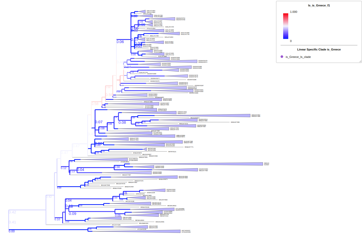
In order to visualize multiple sequence alignment alongside with the tree, first we need to annotate alignment using --alignment in annotate. Then activate alignment layout by adding --alignment-layout
In the previous Functional annotation session we already annotated the tree with multiple sequence alignment, here we will show how to visualize the annotated tree with multiple sequence alignment in examples/pratical_example/emapper.
# Visualize the tree with multiple sequence alignment
treeprofiler plot \
--tree nifH_annotated.ete \
--alignment-layout

--alignment-layout displays multiple sequence alignments with a tree. Whole MSA sequences were visualized with a tree in rectangular layout. Sacle of sequence with position roadmark located at the top.
if metadata is pfam annotations from eggnog-mapper, using --emapper-pfam to annotate domain information in target tree and MUST be with the alignment using --alignment to attach corresponding file.
In order to visualize eggnog-mapper pfam/smart annotations alongside with the tree, first we need to annotate alignment using --emapper-annotations <annotations> in annotate. Then activate alignment layout by adding --emapper-layout.
Once tree is annotated, using --domain-layout to visualize it.
We use example in examples/pratical_example/emapper:
# Visualize the tree with eggnog-mapper pfam/smart annotations
treeprofiler plot \
--tree nifH_annotated.ete \
--domain-layout

domain-layout displays domain annotation with a tree. It requires sequence infomration --alignment in annotate step from MSA sequences to locate domain start and end position.
If metadata is output from eggnog-mapper, using --emapper-annotations automatically parse all information as metadata. Program will parse data of all the columns from emapper output. Once tree is annotated, using --emapper-layout to visualize tree with all the metadata
seed_ortholog evalue score eggNOG_OGs max_annot_lvl COG_category Description Preferred_name GOs EC KEGG_ko KEGG_Pathway KEGG_Module KEGG_Reaction KEGG_rclass BRITE KEGG_TC CAZy BiGG_Reaction PFAMs
We use example in examples/pratical_example/emapper:
# Visualize the tree with eggnog-mapper functional annotations
treeprofiler plot \
--tree nifH_annotated.ete \
--emapper-layout \
--column-width 70
General metadata from emapper annotation

Functional profiling (kegg, ko, gos, etc), collapsed internal nodes shown gradient of presence/total percentage.


If target tree was annotated with --taxon-column in previous annotate step successfully, now activate Taxonomic layout using the following arguments to visualize taxonomic classification. All rank levels will be generated separately and users can switch each of them on/off.
| Argument | Description |
|---|---|
--taxonclade-layout |
Activate taxonclade-layout where clades will be colored based on the taxonomy of each node. |
--taxonrectangle-layout |
Activate taxonrectangle-layout where the taxonomy of each node will be displayed as rectangular blocks in the aligned panel. |
--taxoncollapse-layout |
Activate taxoncollapse-layout where the taxonomy of each node will be displayed as rectangular blocks in the aligned panel, and nodes will be automatically collapsed. |
Only tree which was conducted with taxonomic annotation from treeprofiler in previous annotate step can use the taxonomic visualization.
--taxonclade-layout will assign different color to each taxa from each rank. Each rank will be a individual layout.
we use example in examples/taxonomy_example:
# Visualize the pre-annotated example archaea tree with taxonomic classification
treeprofiler plot \
--tree archaea_annotated.nw \
--taxonclade-layout

--taxonrectangle-layout shows taxonomic classification as rectangular block from root to leaf.
we use example in examples/taxonomy_example:
# Visualize the pre-annotated example archaea tree with taxonomic classification
treeprofiler plot \
--tree archaea_annotated.nw \
--taxonrectangle-layout

--taxoncollapse-layout is similar to --taxonrectangle-layout, but it only show commen ancestor on one column in aligned panel which is shown as corresponding taxa from the rank. Users can switch which layout of rank to be visualized in control panel, once layout of rank is activated, tree will be collapsed based on the according rank. It is more accurate than --taxonrectangle-layout because it also shown the representative taxa in corresponding rank.
we use example in examples/taxonomy_example:
# Visualize the pre-annotated example archaea tree with taxonomic classification
treeprofiler plot \
--tree archaea_annotated.nw \
--taxoncollapse-layout
Collapse at phylumn level:

Collapse at order level:

treeprofiler provides the option to cusomize the color on layouts:
| Argument | Description |
|---|---|
--color-config COLOR_CONFIG |
Path to the file to find the color for each variable. [default: None]. |
-s CONFIG_SEP, --config-sep CONFIG_SEP |
Column separator of color table. [default: \t]. |
A basic template of color.config that you can find in examples/custom_color/color.config.template
# TreeProfiler Color Configuration
# This file defines custom colors for properties of annotated tree nodes.
# Columns: PROP, VALUE, COLOR, CONDITION
# tab-limited or comman-limited

# PROP: Property of the annotated tree node
# VALUE: Value of the property to be colored
# COLOR: Color to apply. Using hex code or word
# CONDITION: Special case for numerical values (optional, e.g., COLOR_MIN, COLOR_MAX, COLOR_MID)

PROP,VALUE,COLOR,CONDITION
| Description | Details |
|---|---|
| PROP | Property of the annotated tree node |
| VALUE | Value of the property to be colored |
| COLOR | Color to apply |
| CONDITION | Special case for numerical values (optional, e.g., COLOR_MIN, COLOR_MAX, COLOR_MID, BARPLOT_COLORBY) |
Here we will use the example from examples/custom_color , where the tree basic_example1.nw is annotated with basic_example1_metadata1.tsv and basic_example1_metadata2.tsv. Therefore the output tree is basic_example1_annotated.ete and basic_example1_annotated.nw.
Check metadata
head -5 basic_example1_metadata1.tsv basic_example1_metadata2.tsv
==> basic_example1_metadata1.tsv <==
#name       sample1 sample2 sample3 sample4 sample5 random_type     bool_type       bool_type2
Phy003I7ZJ_CHICK    0.05    0.12    0.86    0.01    0.69    medium  1       TRUE
Phy0054BO3_MELGA    0.64    0.67    0.51    0.29    0.14    medium  1       TRUE
Phy00508FR_NIPNI    0.89    0.38    0.97    0.49    0.26    low     1       FALSE
Phy004O1E0_APTFO    0.1     0.09    0.38    0.31    0.41    medium  0       TRUE


==> basic_example1_metadata2.tsv <==
#name       abs_data        list_data       abs_data2
Phy003I7ZJ_CHICK    97      w,t,t   50
Phy0054BO3_MELGA    16      r,q,s   245
Phy00508FR_NIPNI    87      z,f,p   122
Phy004O1E0_APTFO    6       z,t,b   138
Column random_type from the metadata is annotated as categorical data property called random_type in result tree basic_example1_annotated.nw. By default, all variables in col6 are: high, medium and low, so let’s customize the in color.categorical.config file:
# TreeProfiler Color Configuration
# This file defines custom colors for properties of annotated tree nodes.
# Columns: PROP, VALUE, COLOR, CONDITION
# tab-limited or comman-limited

# PROP: Property of the annotated tree node
# VALUE: Value of the property to be colored
# COLOR: Color to apply
# CONDITION: Special case for numerical values (optional, e.g., COLOR_MIN, COLOR_MAX, COLOR_MID)

PROP,VALUE,COLOR,CONDITION
random_type,high,red,
random_type,medium,blue,
random_type,low,#008000,
here we can apply this color config to all the layouts for categorical data, for example:
treeprofiler plot \
-t basic_example1_annotated.ete \
--rectangle-layout random_type \
--label-layout random_type \
--background-layout random_type \
--colorbranch-layout random_type \
--piechart-layout random_type \
--color-config color.categorical.config \
-s ,
Now all the layout will be colored based on the color config file.

Noted that if the value is not in the color config file, the default color black will be used.
Missing low value in the color config file:
# TreeProfiler Color Configuration
# This file defines custom colors for properties of annotated tree nodes.
# Columns: PROP, VALUE, COLOR, CONDITION
# tab-limited or comman-limited

# PROP: Property of the annotated tree node
# VALUE: Value of the property to be colored
# COLOR: Color to apply
# CONDITION: Special case for numerical values (optional, e.g., COLOR_MIN, COLOR_MAX, COLOR_MID)

PROP,VALUE,COLOR,CONDITION
random_type,high,red,
random_type,medium,blue,
rerun the command:
treeprofiler plot \
-t basic_example1_annotated.ete \
--rectangle-layout random_type \
--label-layout random_type \
--background-layout random_type \
--colorbranch-layout random_type \
--piechart-layout random_type \
--color-config color.categorical.config \
-s ,

Column bool_type and bool_type2 are boolean data, therefore users can only decide the color representing True value. We stored the following config in color.boolean.config
# TreeProfiler Color Configuration
# This file defines custom colors for properties of annotated tree nodes.
# Columns: PROP, VALUE, COLOR, CONDITION
# tab-limited or comman-limited

# PROP: Property of the annotated tree node
# VALUE: Value of the property to be colored
# COLOR: Color to apply
# CONDITION: Special case for numerical values (optional, e.g., COLOR_MIN, COLOR_MAX, COLOR_MID)

PROP,VALUE,COLOR,CONDITION
bool_type,1,blue,
bool_type2,TRUE,yellow,
Now we appiled them to the layouts for boolean data:
treeprofiler plot \
-t basic_example1_annotated.ete \
--binary-layout bool_type bool_type2 \
--color-config color.boolean.config \
-s ,

We applied the color config to layouts for numerical data in color.numerical.config.
We can still customize certain color for specific value.
For example, we want to make make the heatmap layout with yellow color when value is 0:
# TreeProfiler Color Configuration
# This file defines custom colors for properties of annotated tree nodes.
# Columns: PROP, VALUE, COLOR, CONDITION

# PROP: Property of the annotated tree node
# VALUE: Value of the property to be colored
# COLOR: Color to apply
# CONDITION: Special case for numerical values (optional, e.g., COLOR_MIN, COLOR_MAX, COLOR_MID, COLOR_NAN)

PROP,VALUE,COLOR,CONDITION
sample1,0,yellow,
sample2,0,yellow,
sample3,0,yellow,
sample4,0,yellow,
sample5,0,yellow,
Then we run it on heatmap layout:
treeprofiler plot \
--tree basic_example1_annotated.ete \
--heatmap-layout sample1 sample2 sample3 sample4 sample5 \
--color-config color.numerical.config \
-s ,

Similar on numerical matrix:
treeprofiler plot \
--tree basic_example1_annotated.ete \
--numerical-matrix-layout sample1 sample2 sample3 sample4 sample5 \
--color-config color.numerical.config \
-s ,

In the Basic setting, we only set the color for specific value, but in the Advanced setting, we can set the color for the range of value.
We can set the color range using COLOR_MIN, COLOR_MAX, COLOR_MID or COLOR_NAN under the column CONDITION.
Here we set the color for the range of value in color.numerical2.config, noted that now the VALUE column is empty therefore the maximum value will be assigned to COLOR_MAX, the minimum value will be assigned to COLOR_MIN, and the middle value will be assigned to COLOR_MID:
# TreeProfiler Color Configuration
# This file defines custom colors for properties of annotated tree nodes.
# Columns: PROP, VALUE, COLOR, CONDITION

# PROP: Property of the annotated tree node
# VALUE: Value of the property to be colored
# COLOR: Color to apply
# CONDITION: Special case for numerical values (optional, e.g., COLOR_MIN, COLOR_MAX, COLOR_MID)

PROP,VALUE,COLOR,CONDITION
sample1,,red,COLOR_MAX
sample1,,green,COLOR_MID
sample1,,blue,COLOR_MIN
we run it on heatmap layout:
treeprofiler plot \
--tree basic_example1_annotated.ete \
--heatmap-layout sample1 sample2 sample3 sample4 sample5 \
--color-config color.numerical2.config \
-s ,
As you see, the color is assigned based on the range of value of property sample1:

In the previous example, we set the color range for the values, the value range is the range of minimum and maximum value by default, but we can also cusomize the value together with the color conditions
Here we set the color for the range of value in color.numerical3.config, noted that now the VALUE column is not empty as we set the range from -5 to 5, therefore the value will be assigned to the corresponding color:
# TreeProfiler Color Configuration
# This file defines custom colors for properties of annotated tree nodes.
# Columns: PROP, VALUE, COLOR, CONDITION

# PROP: Property of the annotated tree node
# VALUE: Value of the property to be colored
# COLOR: Color to apply
# CONDITION: Special case for numerical values (optional, e.g., COLOR_MIN, COLOR_MAX, COLOR_MID)

PROP,VALUE,COLOR,CONDITION
sample1,5,red,COLOR_MAX
sample1,0,green,COLOR_MID
sample1,-5,blue,COLOR_MIN
Then we run it on heatmap-layout:
treeprofiler plot \
--tree basic_example1_annotated.ete \
--heatmap-layout sample1 sample2 sample3 sample4 sample5 \
--color-config color.numerical3.config \
-s ,

If we only want to set the range of value without customize the color, is also possible:
Here we want to set up the range from -5 to 5, but we only set them as CONDITION without setting specific color in COLOR column:
# TreeProfiler Color Configuration
# This file defines custom colors for properties of annotated tree nodes.
# Columns: PROP, VALUE, COLOR, CONDITION

# PROP: Property of the annotated tree node
# VALUE: Value of the property to be colored
# COLOR: Color to apply
# CONDITION: Special case for numerical values (optional, e.g., COLOR_MIN, COLOR_MAX, COLOR_MID)

PROP,VALUE,COLOR,CONDITION
sample1,5,,COLOR_MAX
sample1,0,,COLOR_MID
sample1,-5,,COLOR_MIN
Rerun:
treeprofiler plot \
--tree basic_example1_annotated.ete \
--heatmap-layout sample1 sample2 sample3 sample4 sample5 \
--color-config color.numerical3.config \
-s ,

In the session of Layouts for numerical data, we describe the difference between --heatmap-layout and --numerical-matrix-layout. In short, --heatmap-layout treat each property individually therefore the range each column of heatmap is different, but --numerical-matrix-layout treat the whole matrix as a single property, therefore the range of value is the same for all columns.
Therefore, when we set the color config for the numerical matrix layout, we can use the wildcard * to represent all the columns in the matrix.
Here we set the color for the range of value in color.datamatrix.config, noted that now the PROP column is * which means all the columns in the matrix, therefore the value will be assigned to the corresponding color:
# TreeProfiler Color Configuration
# This file defines custom colors for properties of annotated tree nodes.
# Columns: PROP, VALUE, COLOR, CONDITION

# PROP: Property of the annotated tree node
# VALUE: Value of the property to be colored
# COLOR: Color to apply
# CONDITION: Special case for numerical values (optional, e.g., COLOR_MIN, COLOR_MAX, COLOR_MID)

PROP,VALUE,COLOR,CONDITION
*,5,red,COLOR_MAX
*,0,white,COLOR_MID
*,-5,blue,COLOR_MIN
now we run it on numerical-matrix-layout:
treeprofiler plot \
--tree basic_example1_annotated.ete \
--numerical-matrix-layout sample1 sample2 sample3 sample4 sample5 \
--color-config color.datamatrix.config \
-s ,

It applied in also for data matrix properties:
Here we annotate and plot the data_2col.array(a data matrix file) to demo tree demo1.tree:
treeprofiler annotate \
-t demo1.tree \
--data-matrix data_2col.array \
-s , \
-o ./

treeprofiler plot \
-t demo1_annotated.ete \
--numerical-matrix-layout data_2col.array \
--color-config color.datamatrix.config \
-s ,

TreeProfiler allows users to perform conditional process based on different circumstances
| Command Option | Subcommand Availability | Description |
|---|---|---|
--pruned-by |
annotate, plot | Prunes the annotated tree based on specific conditions, removing branches or clades that do not meet the criteria. |
--rank-limit |
annotate, plot | Enables pruning of a taxonomically annotated tree based on the rank of classification. |
--collapsed-by |
plot | Allows users to collapse tree branches based on custom conditions, mainly focusing on internal nodes. |
--highlighted-by |
plot | Enables users to highlight tree nodes that meet specific conditions. |
--internal-plot-measure {sum,avg,max,min,std,none} |
plot | Statistic measures to be shown in numerical layout for internal nodes. [default: avg]. |
In this session we will use examples in examples/automatic_query
| Left Value | Operator | Right Value | |
|---|---|---|---|
| Description | This is the property of either a leaf node or an internal node within the tree. It could be any metadata feature linked to the node, such as its taxonomic classification, gene expression levels, or other biological markers. For example, name, sci_name, support. |
This part of the query specifies the relationship between the left and right values. Operators include: =, !=, >, >=, <, <=, and contains. |
This is the custom criterion against which the left value is compared. Depending on the nature of the left value, this could be a numerical figure, a string, or even a list of values. |
Conditional pruning, prune leaf node whose name contain “FALPE”:
## annotate tree
treeprofiler annotate \
--tree basic_example1.nw \
--metadata ./basic_example1_metadata1.tsv \
--counter-stat relative \
-o ./

# Conditional pruning, prune leaf node whose name contain "FALPE"
treeprofiler plot \
--tree basic_example1_annotated.nw \
--pruned-by "name contains FALPE"
Left panel is tree before prune, right panel is result after prune

## annotate tree
treeprofiler annotate \
--tree basic_example1.nw \
--metadata ./basic_example1_metadata1.tsv \
--counter-stat relative \
-o ./

# select tree node whose name contains `FALPE` character
treeprofiler plot \
--tree basic_example1_annotated.nw \
--input-type newick \
--highlighted-by "name contains FALPE"

The same annotated tree, but select tree node whose sample1 feature > 0.50, here we using ete format which can resume the datatype:
treeprofiler plot \
--tree basic_example1_annotated.ete \
--highlighted-by "sample1 > 0.50" \
--heatmap-layout sample1
if use tree in newick format, we need to attach the prop2type file which can resume the datatype:
treeprofiler plot \
--tree basic_example1_annotated.nw \
--input-type newick \
--prop2type basic_example1_prop2type.txt \
--highlighted-by "sample1 > 0.50" \
--heatmap-layout sample1

Query in internal nodes' properties is also available, in this case, left_value of query will be the internal node property, remember to add the proper suffixes such as _avg, _max,etc, for the numerical data or _counter for categorical and boolean data.
Example
# select tree internal node where sample1_avg feature < 0.50
treeprofiler plot \
--tree basic_example1_annotated.ete \
--collapsed-by "sample1_avg < 0.50" \
--heatmap-layout sample1
 Syntax for internal node counter data
# collapse tree internal nodes, where `high` relative counter > 0.35 in random_type_counter property
treeprofiler plot \
--tree basic_example1_annotated.ete \
--input-type ete \
--rectangle-layout random_type \
--collapsed-by "random_type_counter:high > 0.35" \
--column-width 70

The syntax for the AND condition and OR condition in TreeProfiler is:
AND condition will be under one argument, syntax seperated by ,, such as
# select tree  node where sample1 feature > 0.50 AND sample2 < 0.2
treeprofiler plot \
--tree basic_example1_annotated.ete \
--input-type ete \
--heatmap-layout sample1 sample2 sample3 sample4 sample5 \
--highlighted-by "sample1>0.50,sample2<0.2"
 OR condition will be used more than one arguments
# select tree node where sample1 feature > 0.50 OR sample2 < 0.2
treeprofiler plot \
--tree basic_example1_annotated.ete \
--input-type ete \
--heatmap-layout sample1 sample2 sample3 sample4 sample5 \
--highlighted-by "sample1>0.50" \
--highlighted-by "sample2<0.2"

In conditinary query, it also accept to use config to customize the highlighted and collapsed visualization. Example config file in color.config.template. It has the same structure as color config but the CONDITION column here is for operators as we mentioned in previous session.
cat color.config.template`
# TreeProfiler Conditional query Configuration
# This file defines custom colors for properties of annotated tree nodes.
# Columns: PROP, VALUE, COLOR, CONDITION

# PROP: Property of the annotated tree node
# VALUE: Value of the property to be colored
# COLOR: Color to apply
# CONDITION: operator

PROP,VALUE,COLOR,CONDITION
we use example of basic_example1.nw and basic_example1_metadata1.tsv, we hope to highlight nodes whose random_type is low AND sample1 greater than 0.50, and we want to highlight those nodes in red.
First we customize the config color.config.query:
# TreeProfiler Conditional query Configuration
# This file defines custom colors for properties of annotated tree nodes.
# Columns: PROP, VALUE, COLOR, CONDITION

# PROP: Property of the annotated tree node
# VALUE: Value of the property to be colored
# COLOR: Color to apply
# CONDITION: operator

PROP,VALUE,COLOR,CONDITION
random_type,low,red,=
sample1,0.50,red,>
we attach the config using the same --highlighted-by, dont forget about the -s to indicate the seperator
treeprofiler plot \
-t basic_example1_annotated.ete \
--highlighted-by color.config.query \
-s ,

Similar to --highlighted-by, in this case we try to collapse the internal nodes whose average of leaf properties sample1 greater than 0.50, with color of green.
The config is in color.config.collapsed
# TreeProfiler Conditional query Configuration
# This file defines custom colors for properties of annotated tree nodes.
# Columns: PROP, VALUE, COLOR, CONDITION

# PROP: Property of the annotated tree node
# VALUE: Value of the property to be colored
# COLOR: Color to apply
# CONDITION: operator

PROP,VALUE,COLOR,CONDITION
#random_type_counter:high,0.35,red,>
sample1_avg,0.50,green,>
example run
treeprofiler plot \
-t basic_example1_annotated.ete \
--collapsed-by color.config.collapsed \
-s ,

Prune taxonomic annotated tree based on following taxonomic rank level,
kingdom, phylum, class, order, family, genus, species, subspecies
case in GTDB in examples/taxonomy_example/:
# Case in GTDB
# before pruning
treeprofiler plot \
--tree archaea_annotated.ete \
--input-type ete \
--taxonclade-layout
before rank limit

# prune tree in visualization, rank limit to family level
# after pruning
treeprofiler plot \
--tree archaea_annotated.ete \
--input-type ete \
--taxonclade-layout
After rank_limit
 As you see, class branches of target gtdb tree are all pruned and only left the internal branches which rank as class.
Internal nodes of numerical data are process descriptive statistic analysis by default, hence when users collapse any branch, --barplot_layout or --heatmap_layout will demonstrate representative value, avg by default. Representative value can be changed by using --internal-plot-measure.
cd examples/basic_example1/
# select max instead of avg as internal node plotting representative
treeprofiler plot \
--tree basic_example1_annotated.ete \
--heatmap-layout sample1 sample2 sample3 sample4 sample5 \
--internal-plot-measure max
Before collapsed
 After collapsed avg as internal plot measure
 max as internal plot measure

To illustrate the easiness and flexibility of TreeProfiler, we use it to annotate and visualize the version 202 of the GTDB prokaryotic phylogeny, which represents a species tree with 60,000 representative bacterial and archaeal species in here. GTDB provides the tree in plain newick format and massive datatable with various associated to such species. Apart from the metadata provided by the GTDB, here we also include annotations of genomes and species clusters to habitats from proGenomes3(Fullam et al. 2023).
Example can be found in directory ./examples/pratical/gtdb_r202/. We already prepared the gtdb v202 taxonomic tree gtdbv202.nw by merging Bacteria and Archaea trees, detailed steps are included in merge_gtdbtree.py. Based on the difference of computational capacity, complete steps and pipeline can be found in gtdbv202full_demo.sh and gtdbv202lite_demo.sh.
- A glance of habitat information of progenome3
cd examples/pratical/gtdb_r202/

zcat progenome3.tar.gz|head -n 4
progenome3.tsv0000664000175000017500000343216414447266674012351 0ustar  dengdenggtdb_genome_representative	aquatic_habitat	host_associated	soil_habitat
RS_GCF_004210275.1	f	t	f
GB_GCA_014116815.1
RS_GCF_000730245.1	f	t	f
- Download metadata of archaea and bacteria from gtdb
wget https://data.gtdb.ecogenomic.org/releases/release202/202.0/ar122_metadata_r202.tar.gz
wget https://data.gtdb.ecogenomic.org/releases/release202/202.0/bac120_metadata_r202.tar.gz
- GTDB metadata annotation
Considering the size of GTDB metadata and phylogeney, here we provide two pipelines for user to choose base on their computational resources.
- GTDB partial annotation (lightweight), which we will extract only a few of columns from metadata for annotation
# Extract genome_size, protein_count, gc_percentage, ncbi_assembly_level, ncbi_genome_category columns from GTDB metadata
tar -xf ar122_metadata_r202.tar.gz -O | cut -f1,14,89,13,46,56 > ar122_metadata_r202_lite.tsv
tar -xf bac120_metadata_r202.tar.gz -O | cut -f1,14,89,13,46,56 > bac120_metadata_r202_lite.tsv

# start annotation
treeprofiler annotate \
--tree gtdbv202.nw \
--input-type newick \
--metadata \
ar122_metadata_r202_lite.tsv bac120_metadata_r202_lite.tsv progenome3.tar.gz \
--taxon-column name \
--taxadb GTDB \
-o ./
- GTDB full annotation, which requires >6G disk space and >15G RAM memory.
# Annotate metadatas to taxonomic tree(this step may take a few minutes)
treeprofiler annotate \
--tree gtdbv202.nw \
--input-type newick \
--metadata \
ar122_metadata_r202.tar.gz bac120_metadata_r202.tar.gz progenome3.tar.gz \
--taxon-column name \
--taxadb GTDB \
-o ./
- Visualizing annotated GTDB tree with GTDB metadata, which are
-
genome_size -
protein_count -
gc_percentage -
ncbi_assembly_level -
ncbi_genome_categoryand progenome3 habitat information
-
aquatic_habitat -
host_associated -
soil_habitat
treeprofiler plot \
--tree gtdbv202_annotated.ete \
--input-type ete \
--barplot-layout genome_size protein_count \
--heatmap-layout gc_percentage \
---binary-layout aquatic_habitat host_associated soil_habitat \
--rectangle-layout ncbi_assembly_level ncbi_genome_category \
--taxonclade-layout \
--column-width 70
 Here we show the GTDB v202 taxonomy tree (bacteria+archaea, 47894 leaves) in rectangular tree layout, with selected annotated properties which are displayed by order in aligned panel. Numerical data
 genome_size and protein_count are visualized as barplot, gc_percentage is shown as heatmap. Habitat information of progenome3, aquatic_habitat, host_associated and soil_habitat are shown as binary layout. Two categorical data ncbi_assembly_level and ncbi_genome_category are visualized as rectangular layout. In order to improve memory effiency, tree has default collapse level (10) hence multiple leaf nodes are collapsed as default, if nodes are collapsed, aligned layouts represented corresponding values of each property of annotated internal nodes. In this level, taxonclade-layout of the highest classification kingdom is activated, which demonstrate bacteria in salmon, archaea in blue.
 Once zoom into smaller view in tree, collapse level reduces automatically (or manually) to 1, then leaf nodes are dynamically displayed and rendered. Therefore associated layouts are shown as represending values of annotated leaves.
 taxonclade-layout colored leaf nodes in specie rank level.
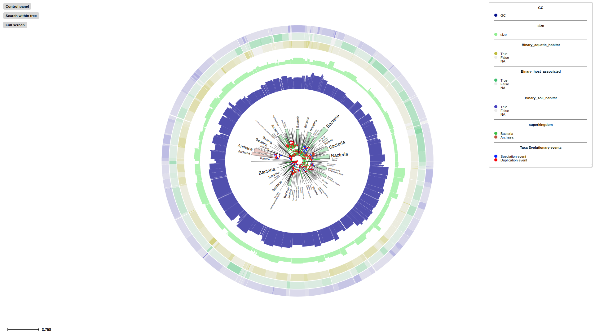 Annotated tree and layouts can be shown as circular tree layout.