
Python package for concise, transparent, and accurate predictive modeling. All sklearn-compatible and easy to use.
Modern machine-learning models are increasingly complex, often making them difficult to interpret. This package provides a simple interface for fitting and using state-of-the-art interpretable models, all compatible with scikit-learn. These models can often replace black-box models (e.g. random forests) with simpler models (e.g. rule lists) while improving interpretability and computational efficiency, all without sacrificing predictive accuracy! Simply import a classifier or regressor and use the fit and predict methods, same as standard scikit-learn models.
from imodels import BoostedRulesClassifier, FIGSClassifier, SkopeRulesClassifier
from imodels import RuleFitRegressor, HSTreeRegressorCV, SLIMRegressor

model = BoostedRulesClassifier()  # initialize a model
model.fit(X_train, y_train)   # fit model
preds = model.predict(X_test) # predictions: shape is (n_test, 1)
preds_proba = model.predict_proba(X_test) # predicted probabilities: shape is (n_test, n_classes)
print(model) # print the rule-based model

-----------------------------
# the model consists of the following 3 rules
# if X1 > 5: then 80.5% risk
# else if X2 > 5: then 40% risk
# else: 10% riskInstall with pip install imodels (see here for help).
| Model | Reference | Description |
|---|---|---|
| Rulefit rule set | 🗂️, 🔗, 📄 | Fits a sparse linear model on rules extracted from decision trees |
| Skope rule set | 🗂️, 🔗 | Extracts rules from gradient-boosted trees, deduplicates them, then linearly combines them based on their OOB precision |
| Boosted rule set | 🗂️, 🔗, 📄 | Sequentially fits a set of rules with Adaboost |
| Slipper rule set | 🗂️, ㅤㅤ📄 | Sequentially learns a set of rules with SLIPPER |
| Bayesian rule set | 🗂️, 🔗, 📄 | Finds concise rule set with Bayesian sampling (slow) |
| Optimal rule list | 🗂️, 🔗, 📄 | Fits rule list using global optimization for sparsity (CORELS) |
| Bayesian rule list | 🗂️, 🔗, 📄 | Fits compact rule list distribution with Bayesian sampling (slow) |
| Greedy rule list | 🗂️, 🔗 | Uses CART to fit a list (only a single path), rather than a tree |
| OneR rule list | 🗂️, ㅤㅤ📄 | Fits rule list restricted to only one feature |
| Optimal rule tree | 🗂️, 🔗, 📄 | Fits succinct tree using global optimization for sparsity (GOSDT) |
| Greedy rule tree | 🗂️, 🔗, 📄 | Greedily fits tree using CART |
| C4.5 rule tree | 🗂️, 🔗, 📄 | Greedily fits tree using C4.5 |
| TAO rule tree | 🗂️, ㅤㅤ📄 | Fits tree using alternating optimization |
| Iterative random forest |
🗂️, 🔗, 📄 | Repeatedly fit random forest, giving features with high importance a higher chance of being selected |
| Sparse integer linear model |
🗂️, ㅤㅤ📄 | Sparse linear model with integer coefficients |
| Greedy tree sums | 🗂️, ㅤㅤ📄 | Sum of small trees with very few total rules (FIGS) |
| Hierarchical shrinkage wrapper |
🗂️, ㅤㅤ📄 | Improve any tree-based model with ultra-fast, post-hoc regularization |
| Distillation wrapper |
🗂️ | Train a black-box model, then distill it into an interpretable model |
| More models | ⌛ | (Coming soon!) Lightweight Rule Induction, MLRules, ... |
Docs 🗂️, Reference code implementation 🔗, Research paper 📄
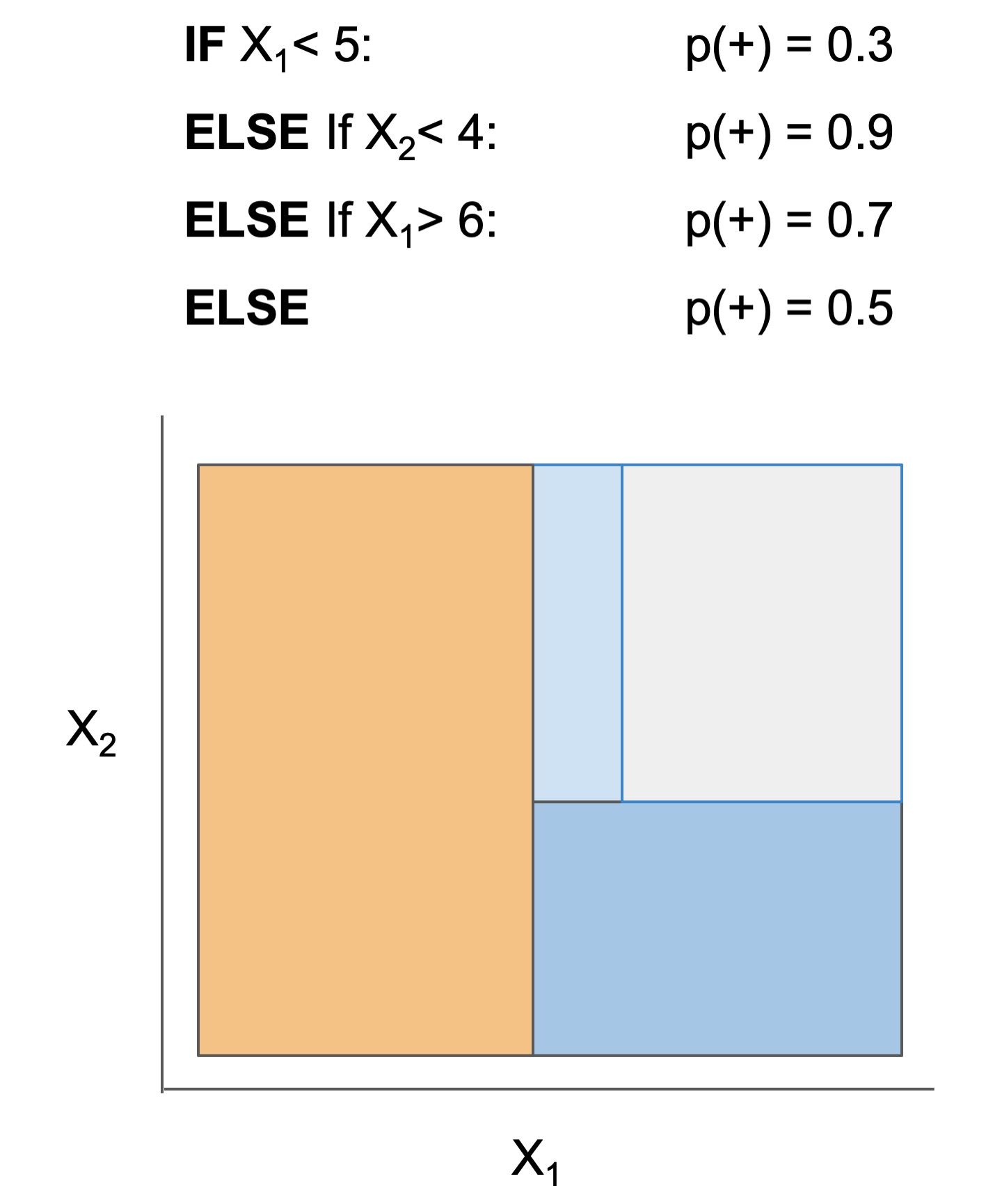
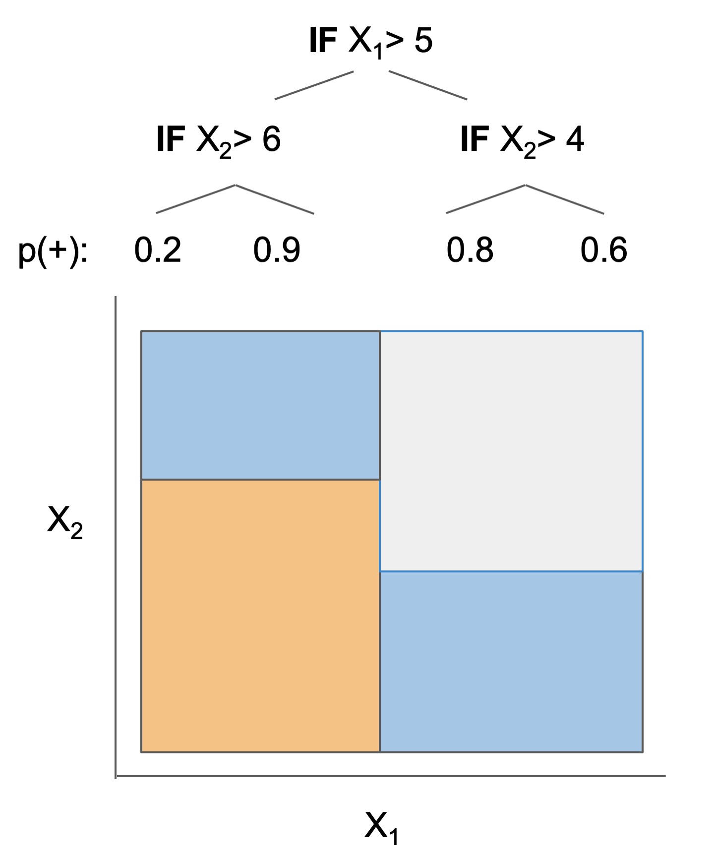
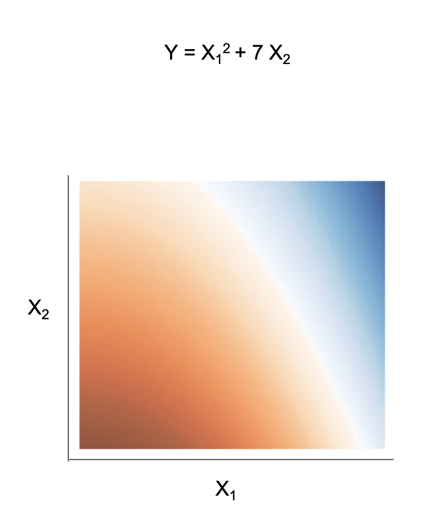
The final form of the above models takes one of the following forms, which aim to be simultaneously simple to understand and highly predictive:
| Rule set | Rule list | Rule tree | Algebraic models |
|---|---|---|---|
 |
 |
 |
 |
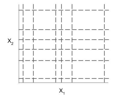
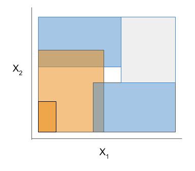
Different models and algorithms vary not only in their final form but also in different choices made during modeling, such as how they generate, select, and postprocess rules:
| Rule candidate generation | Rule selection | Rule postprocessing |
|---|---|---|
 |
 |
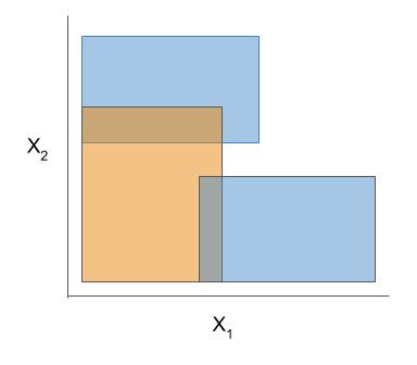 |
Ex. RuleFit vs. SkopeRules
RuleFit and SkopeRules differ only in the way they prune rules: RuleFit uses a linear model whereas SkopeRules heuristically deduplicates rules sharing overlap.Ex. Bayesian rule lists vs. greedy rule lists
Bayesian rule lists and greedy rule lists differ in how they select rules; bayesian rule lists perform a global optimization over possible rule lists while Greedy rule lists pick splits sequentially to maximize a given criterion.Ex. FPSkope vs. SkopeRules
FPSkope and SkopeRules differ only in the way they generate candidate rules: FPSkope uses FPgrowth whereas SkopeRules extracts rules from decision trees.Demos are contained in the notebooks folder.
Quickstart demo
Shows how to fit, predict, and visualize with different interpretable modelsAutogluon demo
Fit/select an interpretable model automatically using Autogluon AutoMLQuickstart colab demo 
Shows how to fit, predict, and visualize with different interpretable models
Clinical decision rule notebook
Shows an example of usingimodels for deriving a clinical decision rule
Posthoc analysis
We also include some demos of posthoc analysis, which occurs after fitting models: posthoc.ipynb shows different simple analyses to interpret a trained model and uncertainty.ipynb contains basic code to get uncertainty estimates for a modelDifferent models support different machine-learning tasks. Current support for different models is given below (each of these models can be imported directly from imodels (e.g. from imodels import RuleFitClassifier):
| Model | Binary classification | Regression | Notes |
|---|---|---|---|
| Rulefit rule set | RuleFitClassifier | RuleFitRegressor | |
| Skope rule set | SkopeRulesClassifier | ||
| Boosted rule set | BoostedRulesClassifier | ||
| SLIPPER rule set | SlipperClassifier | ||
| Bayesian rule set | BayesianRuleSetClassifier | Fails for large problems | |
| Optimal rule list (CORELS) | OptimalRuleListClassifier | Requires corels, fails for large problems | |
| Bayesian rule list | BayesianRuleListClassifier | ||
| Greedy rule list | GreedyRuleListClassifier | ||
| OneR rule list | OneRClassifier | ||
| Optimal rule tree (GOSDT) | OptimalTreeClassifier | Requires gosdt, fails for large problems | |
| Greedy rule tree (CART) | GreedyTreeClassifier | GreedyTreeRegressor | |
| C4.5 rule tree | C45TreeClassifier | ||
| TAO rule tree | TaoTreeClassifier | TaoTreeRegressor | |
| Iterative random forest | IRFClassifier | Requires irf | |
| Sparse integer linear model | SLIMClassifier | SLIMRegressor | Requires extra dependencies for speed |
| Greedy tree sums (FIGS) | FIGSClassifier | FIGSRegressor | |
| Hierarchical shrinkage | HSTreeClassifierCV | HSTreeRegressorCV | Wraps any sklearn tree-based model |
| Distillation | DistilledRegressor | Wraps any sklearn-compatible models |
Data-wrangling functions for working with popular tabular datasets (e.g. compas).
These functions, in conjunction with imodels-data and imodels-experiments, make it simple to download data and run experiments on new models.Explain classification errors with a simple posthoc function.
Fit an interpretable model to explain a previous model's errors (ex. in this notebook📓).Fast and effective discretizers for data preprocessing.
| Discretizer | Reference | Description |
|---|---|---|
| MDLP | 🗂️, 🔗, 📄 | Discretize using entropy minimization heuristic |
| Simple | 🗂️, 🔗 | Simple KBins discretization |
| Random Forest | 🗂️ | Discretize into bins based on random forest split popularity |
Rule-based utils for customizing models
The code here contains many useful and customizable functions for rule-based learning in the util folder. This includes functions / classes for rule deduplication, rule screening, and converting between trees, rulesets, and neural networks.After developing and playing with imodels, we developed a few new models to overcome limitations of existing interpretable models.
Fast Interpretable Greedy-Tree Sums (FIGS) is an algorithm for fitting concise rule-based models. Specifically, FIGS generalizes CART to simultaneously grow a flexible number of trees in a summation. The total number of splits across all the trees can be restricted by a pre-specified threshold, keeping the model interpretable. Experiments across a wide array of real-world datasets show that FIGS achieves state-of-the-art prediction performance when restricted to just a few splits (e.g. less than 20).
Example FIGS model. FIGS learns a sum of trees with a flexible number of trees; to make its prediction, it sums the result from each tree.
Hierarchical shrinkage is an extremely fast post-hoc regularization method which works on any decision tree (or tree-based ensemble, such as Random Forest). It does not modify the tree structure, and instead regularizes the tree by shrinking the prediction over each node towards the sample means of its ancestors (using a single regularization parameter). Experiments over a wide variety of datasets show that hierarchical shrinkage substantially increases the predictive performance of individual decision trees and decision-tree ensembles.
Readings
Reference implementations (also linked above)
The code here heavily derives from the wonderful work of previous projects. We seek to to extract out, unify, and maintain key parts of these projects.- pycorels - by @fingoldin and the original CORELS team
- sklearn-expertsys - by @tmadl and @kenben based on original code by Ben Letham
- rulefit - by @christophM
- skope-rules - by the skope-rules team (including @ngoix, @floriangardin, @datajms, Bibi Ndiaye, Ronan Gautier)
- boa - by @wangtongada
Related packages
- gplearn: symbolic regression/classification
- pysr: fast symbolic regression
- pygam: generative additive models
- interpretml: boosting-based gam
- h20 ai: gams + glms (and more)
- optbinning: data discretization / scoring models
Updates
- For updates, star the repo, see this related repo, or follow @csinva_
- Please make sure to give authors of original methods / base implementations appropriate credit!
- Contributing: pull requests very welcome!
If it's useful for you, please star/cite the package, and make sure to give authors of original methods / base implementations credit:
@software{
    imodels2021,
    title        = {imodels: a python package for fitting interpretable models},
    journal      = {Journal of Open Source Software},
    publisher    = {The Open Journal},
    year         = {2021},
    author       = {Singh, Chandan and Nasseri, Keyan and Tan, Yan Shuo and Tang, Tiffany and Yu, Bin},
    volume       = {6},
    number       = {61},
    pages        = {3192},
    doi          = {10.21105/joss.03192},
    url          = {https://doi.org/10.21105/joss.03192},
}


