Handle missing values, non-numeric values, data leakage, and more.
Introduction in exercise-introduction.ipynb
This course also available on YouTube: George Zoto - Kaggle Mini Courses - Intermediate Machine Learning or by 1littlecoder - Kaggle 30 Days of ML - Day 12 - Kaggle Missing Values, Encoding - Learn Python ML in 30 Days
Unless most values in the dropped columns are missing, the model loses access to a lot of (potentially useful!) information with this approach. As an extreme example, consider a dataset with 10,000 rows, where one important column is missing a single entry. This approach would drop the column entirely!
# Get names of columns with missing values
cols_with_missing = [col for col in X_train.columns
                     if X_train[col].isnull().any()]

# Drop columns in training and validation data
reduced_X_train = X_train.drop(cols_with_missing, axis=1)
reduced_X_valid = X_valid.drop(cols_with_missing, axis=1)

print("MAE from Approach 1 (Drop columns with missing values):")
print(score_dataset(reduced_X_train, reduced_X_valid, y_train, y_valid))
Out:
MAE from Approach 1 (Drop columns with missing values):
183550.22137772635
Imputation fills in the missing values with some number. For instance, we can fill in the mean value along each column.
The imputed value won't be exactly right in most cases, but it usually leads to more accurate models than you would get from dropping the column entirely.
- To make it, use
SimpleImputer()from scikit-learn. You can use parameters such as:strategy=which can be calculated based on each column:mean- replace missing values by the mean along each column, which will be the average of a data setmedian- replace missing values by the median of each column which is the average of a data setmost_frequent- replace missing values with the most frequent values in the column- can be:
constantwhich replace missing values withfill_value
missing_valueswhich set what type will be the replacement:int,float,str,np.nanorNone, by default:default=np.nan
- on the returned table you can use
fit_transform(input_samples)to fit to data, then transform it, and returns a transformed version ofinput_samples- also you can use just
transform(X)which will impute all missing values inXand returnsXwith imputed values.
- also you can use just
For better understanding:
import numpy as np
from sklearn.impute import SimpleImputer

imp_mean = SimpleImputer(missing_values=np.nan, strategy='mean') # For pandas dataframes with nullable integer dtypes
                                                                 # with missing values, missing_values should be set to
                                                                 # np.nan, since pd.NA will be converted to np.nan.
imp_mean.fit([[7, 2, 3], [4, np.nan, 6], [10, 5, 9]])  # Fit the imputer on X
                                                       # now imp_mean is a SimpleImputer()

X = [[np.nan, 2, 3], [4, np.nan, 6], [10, np.nan, 9]]
print(imp_mean.transform(X))
Out:
[[ 7. 2. 3. ]
[ 4. 3.5 6. ]
[10. 3.5 9. ]]
Here we got 3.5 because we used strategy='mean' which calcualtes arithmetic mean of each column, what was in this case the average of column.
In our housing example dataset this will be:
from sklearn.impute import SimpleImputer

# Imputation
my_imputer = SimpleImputer()
imputed_X_train = pd.DataFrame(my_imputer.fit_transform(X_train))
imputed_X_valid = pd.DataFrame(my_imputer.transform(X_valid))

# Imputation removed column names; put them back
imputed_X_train.columns = X_train.columns
imputed_X_valid.columns = X_valid.columns

print("MAE from Approach 2 (Imputation):")
print(score_dataset(imputed_X_train, imputed_X_valid, y_train, y_valid))
Out:
MAE from Approach 2 (Imputation):
178166.46269899711
Imputation is the standard approach, and it usually works well. However, imputed values may be systematically above or below their actual values (which weren't collected in the dataset). Or rows with missing values may be unique in some other way. In that case, your model would make better predictions by considering which values were originally missing.
In this approach, we impute the missing values, as before. And, additionally, for each column with missing entries in the original dataset, we add a new column that shows the location of the imputed entries.
In some cases, this will meaningfully improve results. In other cases, it doesn't help at all.
# Make copy to avoid changing original data (when imputing)
X_train_plus = X_train.copy()
X_valid_plus = X_valid.copy()

# Make new columns indicating what will be imputed
for col in cols_with_missing:
    X_train_plus[col + '_was_missing'] = X_train_plus[col].isnull()
    X_valid_plus[col + '_was_missing'] = X_valid_plus[col].isnull()

# Imputation
my_imputer = SimpleImputer()
imputed_X_train_plus = pd.DataFrame(my_imputer.fit_transform(X_train_plus))
imputed_X_valid_plus = pd.DataFrame(my_imputer.transform(X_valid_plus))

# Imputation removed column names; put them back
imputed_X_train_plus.columns = X_train_plus.columns
imputed_X_valid_plus.columns = X_valid_plus.columns

print("MAE from Approach 3 (An Extension to Imputation):")
print(score_dataset(imputed_X_train_plus, imputed_X_valid_plus, y_train, y_valid))
Out:
MAE from Approach 3 (An Extension to Imputation):
178927.503183954
The training data has 10864 rows and 12 columns, where three columns contain missing data. For each column, less than half of the entries are missing. Thus, dropping the columns removes a lot of useful information, and so it makes sense that imputation would perform better.
more about this in exercise-missing-values.ipynb
- Consider a survey that asks how often you eat breakfast and provides four options: "Never", "Rarely", "Most days", or "Every day". In this case, the data is categorical, because responses fall into a fixed set of categories.
- If people responded to a survey about which what brand of car they owned, the responses would fall into categories like "Honda", "Toyota", and "Ford". In this case, the data is also categorical.
Unfortunately the models can't understand this categories, so we need to transform them.
Using
score_dataset()to compare the three different approaches to dealing with categorical variables. This function reports the mean absolute error (MAE) from a random forest model. Keep in mind: in general, we want the MAE to be as low as possible!On the Melbourne dataset this look like:
Based on data type (
dtype) we obtain a list of all of the categorical variables in the training data. For this dataset, the columns with text indicate categorical variables, these areObjects type now.# Get list of categorical variables s = (X_train.dtypes == 'object') object_cols = list(s[s].index) print("Categorical variables:") print(object_cols)Out: Categorical variables: ['Type', 'Method', 'Regionname']
The easiest approach to dealing with categorical variables is to simply remove them from the dataset. This approach will only work well if the columns did not contain useful information.
We drop the object dtype columns with the select_dtypes() method.
drop_X_train = X_train.select_dtypes(exclude=['object'])
drop_X_valid = X_valid.select_dtypes(exclude=['object'])

print("MAE from Approach 1 (Drop categorical variables):")
print(score_dataset(drop_X_train, drop_X_valid, y_train, y_valid))
Out:
MAE from Approach 1 (Drop categorical variables):
175703.48185157913
Ordinal encoding assigns each unique value to a different integer
Every day  ->   3
never      ->   0
rarely     ->   1
most days  ->   2
never      ->   0
This assumption makes sense in this example, because there is an indisputable ranking to the categories. Not all categorical variables have a clear ordering in the values, but we refer to those that do as ordinal variables. For tree-based models (like decision trees and random forests), you can expect ordinal encoding to work well with ordinal variables.
Scikit-learn has a OrdinalEncoder class that can be used to get ordinal encodings. We loop over the categorical variables and apply the ordinal encoder separately to each column.
For each column, we randomly assign each unique value to a different integer. This is a common approach that is simpler than providing custom labels; however, we can expect an additional boost in performance if we provide better-informed labels for all ordinal variables.
from sklearn.preprocessing import OrdinalEncoder

# Make copy to avoid changing original data
label_X_train = X_train.copy()
label_X_valid = X_valid.copy()

# Apply ordinal encoder to each column with categorical data
ordinal_encoder = OrdinalEncoder()
label_X_train[object_cols] = ordinal_encoder.fit_transform(X_train[object_cols])
label_X_valid[object_cols] = ordinal_encoder.transform(X_valid[object_cols])

print("MAE from Approach 2 (Ordinal Encoding):")
print(score_dataset(label_X_train, label_X_valid, y_train, y_valid))
Out:
MAE from Approach 2 (Ordinal Encoding):
165936.40548390493
One-hot encoding creates new columns indicating the presence (or absence) of each possible value in the original data. To understand this, we'll work through an example.
Color       =>   Red    Yellow    Green
Red               1        0        0
Red               1        0        0
Yellow            0        1        0
Green             0        0        1
Yelow             0        1        0
In the original dataset, "Color" is a categorical variable with three categories: "Red", "Yellow", and "Green". The corresponding one-hot encoding contains one column for each possible value, and one row for each row in the original dataset. Wherever the original value was "Red", we put a 1 in the "Red" column; if the original value was "Yellow", we put a 1 in the "Yellow" column, and so on.
In contrast to ordinal encoding, one-hot encoding does not assume an ordering of the categories. Thus, you can expect this approach to work particularly well if there is no clear ordering in the categorical data (e.g., "Red" is neither more nor less than "Yellow"). We refer to categorical variables without an intrinsic ranking as nominal variables.
One-hot encoding generally does not perform well if the categorical variable takes on a large number of values (i.e., you generally won't use it for variables taking more than 15 different values).
We use the OneHotEncoder class from scikit-learn to get one-hot encodings. There are a number of parameters that can be used to customize its behavior.
used parameters:
handle_unknown='ignore'to avoid errors when the validation data contains classes that aren't represented in the training data, andsparse=Falseensures that the encoded columns are returned as a numpy array (instead of a sparse matrix).
To use the encoder, we supply only the categorical columns that we want to be one-hot encoded. For instance, to encode the training data, we supply X_train[object_cols]. object_cols in the code cell below is a list of the column names with categorical data, and so X_train[object_cols] contains all of the categorical data in the training set.)
from sklearn.preprocessing import OneHotEncoder

# Apply one-hot encoder to each column with categorical data
OH_encoder = OneHotEncoder(handle_unknown='ignore', sparse=False)
OH_cols_train = pd.DataFrame(OH_encoder.fit_transform(X_train[object_cols]))
OH_cols_valid = pd.DataFrame(OH_encoder.transform(X_valid[object_cols]))

# One-hot encoding removed index; put it back
OH_cols_train.index = X_train.index
OH_cols_valid.index = X_valid.index

# Remove categorical columns (will replace with one-hot encoding)
num_X_train = X_train.drop(object_cols, axis=1)
num_X_valid = X_valid.drop(object_cols, axis=1)

# Add one-hot encoded columns to numerical features
OH_X_train = pd.concat([num_X_train, OH_cols_train], axis=1)
OH_X_valid = pd.concat([num_X_valid, OH_cols_valid], axis=1)

print("MAE from Approach 3 (One-Hot Encoding):")
print(score_dataset(OH_X_train, OH_X_valid, y_train, y_valid))
Out:
MAE from Approach 3 (One-Hot Encoding):
166089.4893009678
A critical skill for deploying (and even testing) complex models with pre-processing.
full example of pipelines: kaggle.com/alexisbcook/exercise-pipelines; or exercise-pipelines.ipynb
A simple way to keep your data preprocessing and modeling code organized. Specifically, a pipeline bundles preprocessing and modeling steps so you can use the whole bundle as if it were a single step.
Why to use pipelines:
- Cleaner Code: Accounting for data at each step of preprocessing can get messy. With a pipeline, you won't need to manually keep track of your training and validation data at each step. like on DAGsHub
- Fewer Bugs: There are fewer opportunities to misapply a step or forget a preprocessing step.
- Easier to Productionize: It can be surprisingly hard to transition a model from a prototype to something deployable at scale. We won't go into the many related concerns here, but pipelines can help.
We take a peek at the training data from Melbourne Housing dataset with the head() method below. Notice that the data contains both categorical data and columns with missing values. With a pipeline, it's easy to deal with both!
       Type   Method  Regionname            Rooms   Distance  Postcode  Bedroom2  Bathroom  Car   Landsize  BuildingArea  YearBuilt   Lattitude   Longtitude  Propertycount
12167   u       S     Southern Metropolitan   1       5.0     3182.0      1.0        1.0    1.0   0.0         NaN          1940.0     -37.85984   144.9867     13240.0
6524    h       SA    Western Metropolitan    2       8.0     3016.0      2.0        2.0    1.0   193.0       NaN          NaN        -37.85800   144.9005     6380.0
8413    h       S     Western Metropolitan    3      12.6     3020.0      3.0        1.0    1.0   555.0       NaN          NaN        -37.79880   144.8220     3755.0
2919    u       SP    Northern Metropolitan   3      13.0     3046.0      3.0        1.0    1.0   265.0       NaN          1995.0     -37.70830   144.9158     8870.0
6043    h       S     Western Metropolitan    3      13.3     3020.0      3.0        1.0    2.0   673.0       673.0        1970.0     -37.76230   144.8272     4217.0
We use sklearn.compose.ColumnTransformer to boundle dfferent preprocessing steps:
- impute missing values in numerical data
- impute missing values and applies one-hot encoding in categorial data
from sklearn.compose import ColumnTransformer
from sklearn.pipeline import Pipeline
from sklearn.impute import SimpleImputer
from sklearn.preprocessing import OneHotEncoder

# Preprocessing for numerical data
numerical_transformer = SimpleImputer(strategy='constant')

# Preprocessing for categorical data
categorical_transformer = Pipeline(steps=[
    ('imputer', SimpleImputer(strategy='most_frequent')),
    ('onehot', OneHotEncoder(handle_unknown='ignore'))
])

# Bundle preprocessing for numerical and categorical data
preprocessor = ColumnTransformer(
    transformers=[
        ('num', numerical_transformer, numerical_cols),
        ('cat', categorical_transformer, categorical_cols)
])Using RandomForestRegressor
from sklearn.ensemble import RandomForestRegressor

model = RandomForestRegressor(n_estimators=100, random_state=0)from sklearn.metrics import mean_absolute_error
# Bundle preprocessing and modeling code in a pipeline
my_pipeline = Pipeline(steps=[('preprocessor', preprocessor),
('model', model)
])
# Preprocessing of training data, fit model
my_pipeline.fit(X_train, y_train)
# Preprocessing of validation data, get predictions
preds = my_pipeline.predict(X_valid) # the pipeline automatically preprocesses the features
# before generating predictions.
# (However, without a pipeline, we have to remember
# to preprocess the validation data before making predictions.)
# Evaluate the model
score = mean_absolute_error(y_valid, preds)
print('MAE:', score)Out:
MAE: 160679.18917034855
NOTE: If MAE is too high amend
numerical_transformer,categorical_transformer, and/ormodelto get better performance.In the case of
numerical_transformerandcategorical_transformerthis means that you have to change theSimpleImputer()'sstrategyattribute and/or set up betterfill_valuetoo.In the case of
modelyou can change in theRandomForestRegressor()'sn_estimatorsandrandom_state.
Wikipedia; file: exercise-cross-validation.ipynb
A better way to test your models.
You will face choices about what predictive variables to use, what types of models to use, what arguments to supply to those models, etc. So far, you have made these choices in a data-driven way by measuring model quality with a validation (or holdout) set.
ex: imagine you have a dataset with 5000 rows. You will typically keep about 20% of the data as a validation dataset, or 1000 rows. But this leaves some random chance in determining model scores. That is, a model might do well on one set of 1000 rows, even if it would be inaccurate on a different 1000 rows
Unfortunately, we can only get a large validation set by removing rows from our training data, and smaller training datasets mean worse models!
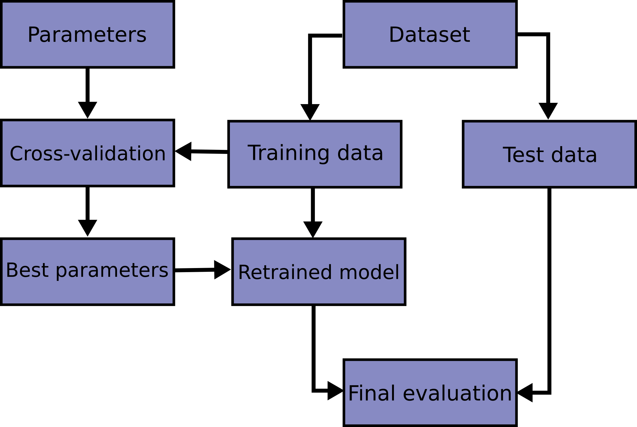
We could begin by dividing the data into 5 pieces, each 20% of the full dataset. In this case, we say that we have broken the data into 5 "folds".
- Experiment 1, we use the first fold as a validation (or holdout) set and everything else as training data. This gives us a measure of model quality based on a 20% holdout set.
- Experiment 2, we hold out data from the second fold (and use everything except the second fold for training the model). The holdout set is then used to get a second estimate of model quality.
- We repeat this process, using every fold once as the holdout set. Putting this together, 100% of the data is used as holdout at some point, and we end up with a measure of model quality that is based on all of the rows in the dataset (even if we don't use all rows simultaneously).
And we can do this on the all dataset:

it can take longer to run, because it estimates multiple models (one for each fold)
when use it:
- For small datasets, where extra computational burden isn't a big deal, you should run cross-validation. If your model takes a couple minutes or less to run, it's probably worth switching to cross-validation.
- For larger datasets, a single validation set is sufficient. Your code will run faster, and you may have enough data that there's little need to re-use some of it for holdout.
We obtain the cross-validation scores with the cross_val_score() function from scikit-learn.
cv- Determines the cross-validation splitting strategy. Possible inputs for cv are:None- by default 5-fold cross validationint- to specify the number of folds in a (Stratified)KFold - usually the higher the worse the result- CV splitter like
train_test_split:clf = svm.SVC(kernel='linear', C=1).fit(X_train, y_train)cross-validation generator- A non-estimator family of classes used to split a dataset into a sequence of train and test portionscross-validation estimatorAn estimator that has built-in cross-validation capabilities to automatically select the best hyper-parameters ex:ElasticNetCV,LogisticRegressionCVscorer- A non-estimator callable object which evaluates an estimator on given test data, returning a number.clf.score(X_test, y_test). higher return values are better than lower return values. If you are usingGridSearchCVorcross_val_scoreyou can setscoringparameter.
scoring- this will quantifying the quality of predictions, you can use predefined values for common use-cases or you can define your scoring strategy from metric functions- An iterable that generates (train, test) splits as arrays of indices, like
train_test_split
- An iterable that generates (train, test) splits as arrays of indices, like
from sklearn.ensemble import RandomForestRegressor
from sklearn.pipeline import Pipeline
from sklearn.impute import SimpleImputer
from sklearn.model_selection import cross_val_score

my_pipeline = Pipeline(steps=[('preprocessor', SimpleImputer()),
                              ('model', RandomForestRegressor(n_estimators=50, # the number of trees in the forest, to optimize it see Hyperparameter optimization problem
                                                              random_state=0)) # Controls the randomness of the bootstrapping
                                                                               # of the samples used when building trees
                                                                               # if bootstrap=True
                             ])

# Multiply by -1 since sklearn calculates *negative* MAE
scores = -1 * cross_val_score(my_pipeline, X, y,
                              cv=5, # get lower for better output
                              scoring='neg_mean_absolute_error') # which is a regressor:
                                                                 # https://scikit-learn.org/stable/modules/generated/sklearn.metrics.mean_absolute_error.html#sklearn.metrics.mean_absolute_error

print("MAE scores:\n", scores)
print("\nAverage MAE score (across experiments):")
print(scores.mean())
Out:
MAE scores:
[301628.7893587 303164.4782723 287298.331666 236061.84754543
260383.45111427]
Average MAE score (across experiments):
277707.3795913405
Using cross-validation yields a much better measure of model quality, with the added benefit of cleaning up our code: note that we no longer need to keep track of separate training and validation sets. So, especially for small datasets, it's a good improvement!
To optimize better values for n_estimators see Hyperparameter optimization and .GridSearcCV for better model selection.
The most accurate modeling technique for structured data.
file: exercise-xgboost.ipynb
Now we are using gradient-boosting insted of random forests.
It begins by initializing the ensemble with a single model, whose predictions can be pretty naive.
Then, we start the cycle:
- we use the current ensemble to generate predictions for each observation in the dataset. To make a prediction, we add the predictions from all models in the ensemble to calculate a loss function (ex: mean squared error).
- Then, we use the loss function to fit a new model that will be added to the ensemble. Specifically, we determine model parameters so that adding this new model to the ensemble will reduce the loss. (Side note: The "gradient" in "gradient boosting" refers to the fact that we'll use gradient descent on the loss function to determine the parameters in this new model. "X" stands for extreme, so this will be extreme gradient boosting)
- Finally, we add the new model to ensemble, and ...
- ... repeat!

for this we will use xgboost.XGBRegressor wehere we also can set
n_estimators- pecifies how many times to go through the modeling cycle described above. It is equal to the number of models that we include in the ensemble- Too low a value causes underfitting
- Too high a value causes overfitting
- Typical values range from
100-1000, though this depends a lot on thelearning_rate
early_stopping_rounds- Early stopping causes the model to stop iterating when the validation score stops improving, at the ideal value forn_estimators. Settingearly_stopping_rounds=5is a reasonable choice. In this case, we stop after 5 straight rounds of deteriorating validation scoreseval_set- we need to set forearly_stopping_roundsfit()values to fit gradient boosting model. This parameter replacesearly_stopping_roundinfit(). The last entry will be used for early stopping! ex: usuallyeval_set=[(X_valid, y_valid)]
verbose- if True writes the evaluation metric measured on the validation set to stderrlearning_rate- instead of getting predictions by simply adding up the predictions from each component model, we can multiply the predictions from each model by a small number before adding them => each tree we add to the ensemble helps us less ! In general, a small learning rate and large number of estimators will yield more accurate XGBoost models, by default this islearning_rate=0.1n_jobs- On larger datasets where runtime is a consideration, you can use parallelism to build your models faster. It's common to set the parametern_jobsequal to the number of cores on your machine. On smaller datasets, this won't help. At Google Collab this is 2, at Kaggle this is 4 at Deepnote 2-16, depends on subscirption at gradient it means 2-8-12 at Datalore this will be an AWS based ec2 t2.medium based VM which has 2 vCPUrandom_state- expose a number of methods for generating random numbers drawn from a variety of probability distributions. In addition to the distribution-specific arguments, each method takes a keyword argument size that defaults to None. A seed can beseed{None, int, array_like, BitGenerator}- and many of parameters like before at
cross_val_score
from xgboost import XGBRegressor
from sklearn.metrics import mean_absolute_error

#my_model = XGBRegressor()
#my_model.fit(X_train, y_train)

my_model = XGBRegressor(n_estimators=1000, learning_rate=0.05, n_jobs=4)
my_model.fit(X_train, y_train,
             early_stopping_rounds=5,
             eval_set=[(X_valid, y_valid)],
             verbose=False)

predictions = my_model.predict(X_valid)
print("Mean Absolute Error: " + str(mean_absolute_error(predictions, y_valid)))
fst Out:
Mean Absolute Error: 239435.01260125183
Find and fix this problem that ruins your model in subtle ways.
Data leakage (or leakage) happens when your training data contains information about the target, but similar data will not be available when the model is used for prediction. This leads to high performance on the training set (and possibly even the validation data), but the model will perform poorly in production.
In other words, leakage causes a model to look accurate until you start making decisions with the model, and then the model becomes very inaccurate.
when your predictors include data that will not be available at the time you make predictions. It is important to think about target leakage in terms of the timing or chronological order that data becomes available, not merely whether a feature helps make good predictions.
An example will be helpful. Imagine you want to predict who will get sick with pneumonia. The top few rows of your raw data look like this:
got_pneumonia   age   weight  male  took_antibiotic_medicine  ...
False           65     100   False    False                   ...
False           72     130   True     False                   ...
True            58     100   False    True                    ...
People take antibiotic medicines after getting pneumonia in order to recover. The raw data shows a strong relationship between those columns, but took_antibiotic_medicine is frequently changed after the value for got_pneumonia is determined. This is target leakage.
- Since validation data comes from the same source as training data, the pattern will repeat itself in validation, and the model will have great validation (or cross-validation) scores.
- But the model will be very inaccurate when subsequently deployed in the real world, because even patients who will get pneumonia won't have received antibiotics yet
Recall that validation is meant to be a measure of how the model does on data that it hasn't considered before. You can corrupt this process in subtle ways if the validation data affects the preprocessing behavior.
ex: run preprocessing (like fitting an imputer for missing values) before calling train_test_split() => Your model may get good validation scores, giving you great confidence in it, but perform poorly when you deploy it to make decisions. This problem becomes even more subtle (and more dangerous) when you do more complex feature engineering.
If your validation is based on a simple train-test split, exclude the validation data from any type of fitting, including the fitting of preprocessing steps. This is easier if you use scikit-learn pipelines. When using cross-validation, it's even more critical that you do your preprocessing inside the pipeline!
We will use a dataset about credit card applications and skip the basic data set-up code. The end result is that information about each credit card application is stored in a DataFrame X. We'll use it to predict which applications were accepted in a Series y.
import pandas as pd

# Read the data
data = pd.read_csv('../input/aer-credit-card-data/AER_credit_card_data.csv',
                   true_values = ['yes'], false_values = ['no'])

# Select target
y = data.card

# Select predictors
X = data.drop(['card'], axis=1)

print("Number of rows in the dataset:", X.shape[0])
X.head()
Out:
Number of rows in the dataset: 1319
reports age income share expenditure owner selfemp dependents months majorcards active
0 0 37.66667 4.5200 0.033270 124.983300 True False 3 54 1 12
1 0 33.25000 2.4200 0.005217 9.854167 False False 3 34 1 13
2 0 33.66667 4.5000 0.004156 15.000000 True False 4 58 1 5
3 0 30.50000 2.5400 0.065214 137.869200 False False 0 25 1 7
4 0 32.16667 9.7867 0.067051 546.503300 True False 2 64 1 5
Since this is a small dataset, we will use cross-validation to ensure accurate measures of model quality.
from sklearn.pipeline import make_pipeline
from sklearn.ensemble import RandomForestClassifier
from sklearn.model_selection import cross_val_score

# Since there is no preprocessing, we don't need a pipeline (used anyway as best practice!)
my_pipeline = make_pipeline(RandomForestClassifier(n_estimators=100))
cv_scores = cross_val_score(my_pipeline, X, y,
                            cv=5,
                            scoring='accuracy')

print("Cross-validation accuracy: %f" % cv_scores.mean())
Out:
Cross-validation accuracy: 0.980292
With experience, you'll find that it's very rare to find models that are accurate 98% of the time. It happens, but it's uncommon enough that we should inspect the data more closely for target leakage.
Here is a summary of the data, which you can also find under the data tab:
card: 1 if credit card application accepted, 0 if notreports: Number of major derogatory reportsage: Age n years plus twelfths of a yearincome: Yearly income (divided by 10,000)share: Ratio of monthly credit card expenditure to yearly incomeexpenditure: Average monthly credit card expenditureowner: 1 if owns home, 0 if rentsselfempl: 1 if self-employed, 0 if notdependents: 1 + number of dependentsmonths: Months living at current addressmajorcards: Number of major credit cards heldactive: Number of active credit accounts
A few variables look suspicious. ex: does expenditure mean expenditure on this card or on cards used before appying?
At this point, basic data comparisons can be very helpful:
expenditures_cardholders = X.expenditure[y]
expenditures_noncardholders = X.expenditure[~y]

print('Fraction of those who did not receive a card and had no expenditures: %.2f' \
      %((expenditures_noncardholders == 0).mean()))
print('Fraction of those who received a card and had no expenditures: %.2f' \
      %(( expenditures_cardholders == 0).mean()))
Out:
Fraction of those who did not receive a card and had no expenditures: 1.0
0
Fraction of those who received a card and had no expenditures: 0.02
everyone who did not receive a card had no expenditures, while only 2% of those who received a card had no expenditures?
now we exclude:
share- is partially determined byexpenditureactiveandmajorcards- less clear
# Drop leaky predictors from dataset
potential_leaks = ['expenditure', 'share', 'active', 'majorcards']
X2 = X.drop(potential_leaks, axis=1)

# Evaluate the model with leaky predictors removed
cv_scores = cross_val_score(my_pipeline, X2, y,
                            cv=5,
                            scoring='accuracy')

print("Cross-val accuracy: %f" % cv_scores.mean())
Out:
Cross-val accuracy: 0.838510
This accuracy is quite a bit lower, which might be disappointing. However, we can expect it to be right about 80% of the time when used on new applications, whereas the leaky model would likely do much worse than that (in spite of its higher apparent score in cross-validation).
Nike has hired you as a data science consultant to help them save money on shoe materials. Your first assignment is to review a model one of their employees built to predict how many shoelaces they'll need each month. The features going into the machine learning model include:
- The current month (January, February, etc)
- Advertising expenditures in the previous month
- Various macroeconomic features (like the unemployment rate) as of the beginning of the current month
- The amount of leather they ended up using in the current month
The results show the model is almost perfectly accurate if you include the feature about how much leather they used. But it is only moderately accurate if you leave that feature out. You realize this is because the amount of leather they use is a perfect indicator of how many shoes they produce, which in turn tells you how many shoelaces they need.
Do you think the leather used feature constitutes a source of data leakage? If your answer is "it depends," what does it depend on?
Answer:
This is tricky, and it depends on details of how data is collected (which is common when thinking about leakage). Would you at the beginning of the month decide how much leather will be used that month? If so, this is ok. But if that is determined during the month, you would not have access to it when you make the prediction. If you have a guess at the beginning of the month, and it is subsequently changed during the month, the actual amount used during the month cannot be used as a feature (because it causes leakage).
You have a new idea. You could use the amount of leather Nike ordered (rather than the amount they actually used) leading up to a given month as a predictor in your shoelace model.
Does this change your answer about whether there is a leakage problem? If you answer "it depends," what does it depend on?
Answer:
This could be fine, but it depends on whether they order shoelaces first or leather first. If they order shoelaces first, you won't know how much leather they've ordered when you predict their shoelace needs. If they order leather first, then you'll have that number available when you place your shoelace order, and you should be ok.
You saved Nike so much money that they gave you a bonus. Congratulations.
Your friend, who is also a data scientist, says he has built a model that will let you turn your bonus into millions of dollars. Specifically, his model predicts the price of a new cryptocurrency (like Bitcoin, but a newer one) one day ahead of the moment of prediction. His plan is to purchase the cryptocurrency whenever the model says the price of the currency (in dollars) is about to go up.
The most important features in his model are:
- Current price of the currency
- Amount of the currency sold in the last 24 hours
- Change in the currency price in the last 24 hours
- Change in the currency price in the last 1 hour
- Number of new tweets in the last 24 hours that mention the currency
The value of the cryptocurrency in dollars has fluctuated up and down by over $100 in the last year, and yet his model's average error is less than $1. He says this is proof his model is accurate, and you should invest with him, buying the currency whenever the model says it is about to go up.
Is he right? If there is a problem with his model, what is it?
Answer:
There is no source of leakage here. These features should be available at the moment you want to make a predition, and they're unlikely to be changed in the training data after the prediction target is determined. But, the way he describes accuracy could be misleading if you aren't careful. If the price moves gradually, today's price will be an accurate predictor of tomorrow's price, but it may not tell you whether it's a good time to invest. For instance, if it is 100𝑡𝑜𝑑𝑎𝑦,𝑎𝑚𝑜𝑑𝑒𝑙𝑝𝑟𝑒𝑑𝑖𝑐𝑡𝑖𝑛𝑔𝑎𝑝𝑟𝑖𝑐𝑒𝑜𝑓100 tomorrow may seem accurate, even if it can't tell you whether the price is going up or down from the current price. A better prediction target would be the change in price over the next day. If you can consistently predict whether the price is about to go up or down (and by how much), you may have a winning investment opportunity.
An agency that provides healthcare wants to predict which patients from a rare surgery are at risk of infection, so it can alert the nurses to be especially careful when following up with those patients.
You want to build a model. Each row in the modeling dataset will be a single patient who received the surgery, and the prediction target will be whether they got an infection.
Some surgeons may do the procedure in a manner that raises or lowers the risk of infection. But how can you best incorporate the surgeon information into the model?
You have a clever idea.
- Take all surgeries by each surgeon and calculate the infection rate among those surgeons.
- For each patient in the data, find out who the surgeon was and plug in that surgeon's average infection rate as a feature.
Does this pose any target leakage issues? Does it pose any train-test contamination issues?
Answer:
This poses a risk of both target leakage and train-test contamination (though you may be able to avoid both if you are careful).
You have target leakage if a given patient's outcome contributes to the infection rate for his surgeon, which is then plugged back into the prediction model for whether that patient becomes infected. You can avoid target leakage if you calculate the surgeon's infection rate by using only the surgeries before the patient we are predicting for. Calculating this for each surgery in your training data may be a little tricky.
You also have a train-test contamination problem if you calculate this using all surgeries a surgeon performed, including those from the test-set. The result would be that your model could look very accurate on the test set, even if it wouldn't generalize well to new patients after the model is deployed. This would happen because the surgeon-risk feature accounts for data in the test set. Test sets exist to estimate how the model will do when seeing new data. So this contamination defeats the purpose of the test set.
You will build a model to predict housing prices. The model will be deployed on an ongoing basis, to predict the price of a new house when a description is added to a website.
Here are four features that could be used as predictors.
- Size of the house (in square meters)
- Average sales price of homes in the same neighborhood
- Latitude and longitude of the house
- Whether the house has a basement
You have historic data to train and validate the model. Which of the features is most likely to be a source of leakage?
Answer:
- 2 is the source of target leakage. Here is an analysis for each feature:
- 1 The size of a house is unlikely to be changed after it is sold (though technically it's possible). But typically this will be available when we need to make a prediction, and the data won't be modified after the home is sold. So it is pretty safe.
- 2 We don't know the rules for when this is updated. If the field is updated in the raw data after a home was sold, and the home's sale is used to calculate the average, this constitutes a case of target leakage. At an extreme, if only one home is sold in the neighborhood, and it is the home we are trying to predict, then the average will be exactly equal to the value we are trying to predict. In general, for neighborhoods with few sales, the model will perform very well on the training data. But when you apply the model, the home you are predicting won't have been sold yet, so this feature won't work the same as it did in the training data.
- 3 These don't change, and will be available at the time we want to make a prediction. So there's no risk of target leakage here.
- 4 This also doesn't change, and it is available at the time we want to make a prediction. So there's no risk of target leakage here.