Demo site: https://quickomics.bxgenomics.com
Tutorial with supplementary tables: https://bit.ly/3rXIyhL
Online Tutorial of Ver. 2: https://interactivereport.github.io/Quickomics/tutorial/docs/
Cite: Gao B, Zhu J, Negi S, Zhang X, Gyoneva S, Casey F, Wei R, Zhang B. Quickomics: exploring omics data in an intuitive, interactive and informative manner. Bioinformatics. 2021 Apr 26:btab255. https://doi.org/10.1093/bioinformatics/btab255
BioRxiv preprint: https://www.biorxiv.org/content/10.1101/2021.01.19.427296v2
Interactive Figure 1: https://interactivereport.github.io/Quickomics/Figure1.html
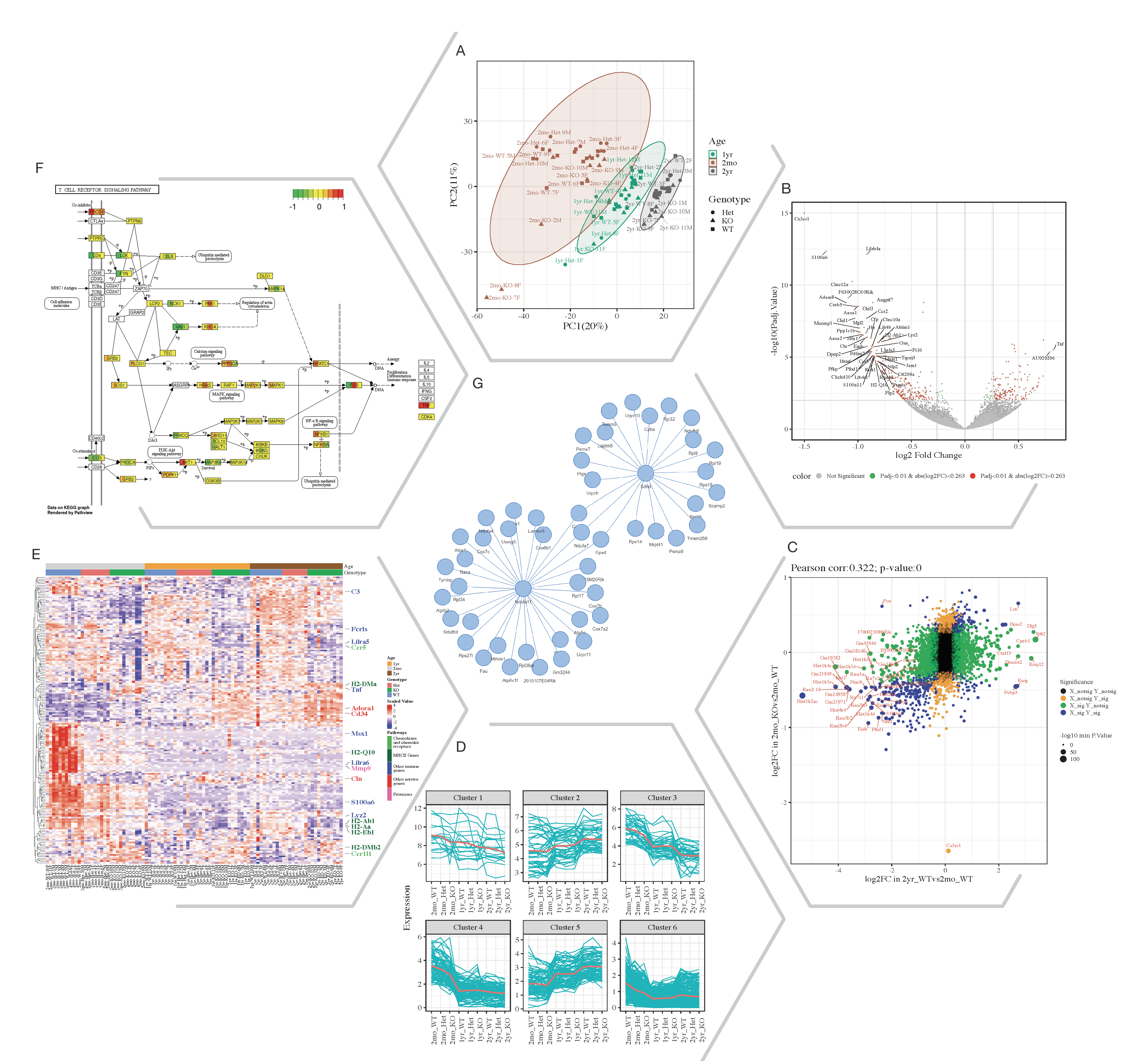
Fig. 1. Selected Quickomics functions applied to a dataset of microglial RNA-seq gene expression from three mouse genotypes over time. A) PCA based on full dataset highlights primary sample separation by mouse age at which the cells were isolated. (B) Volcano plot visualizes differentially expressed genes, most of which show reduced expression in 2mo KO compared to 2mo_WT microglia. For spacing purpose, absolute log2FC (Fold Change) and negative log10 adjusted p-value are capped at 1.5 and 15, respectively. (C) Correlation analysis between two comparisons shows that aging and Cx3cr1-KO have a similar effect on gene expression. (D) Pattern clustering identifies subsets of genes with similar expression over the samples. The clustering is mostly driven by age, with the KO genotype having a similar, but smaller effect. (E) Heatmap of all samples allows the identification of gene clusters with expression regulated by age and/or genotype. Key genes and the pathways they belong to are highlighted on the right. (F) After pathway enrichment analysis, KEGG pathways (Kanehisa and Goto, 2000) of interest can be displayed in a cellular context. The color bars with each stripe representing one comparison show log2 fold changes in various comparisons, allowing project-wide insights for patterns of expression. (G) Correlation network shows potential links between genes of interest.
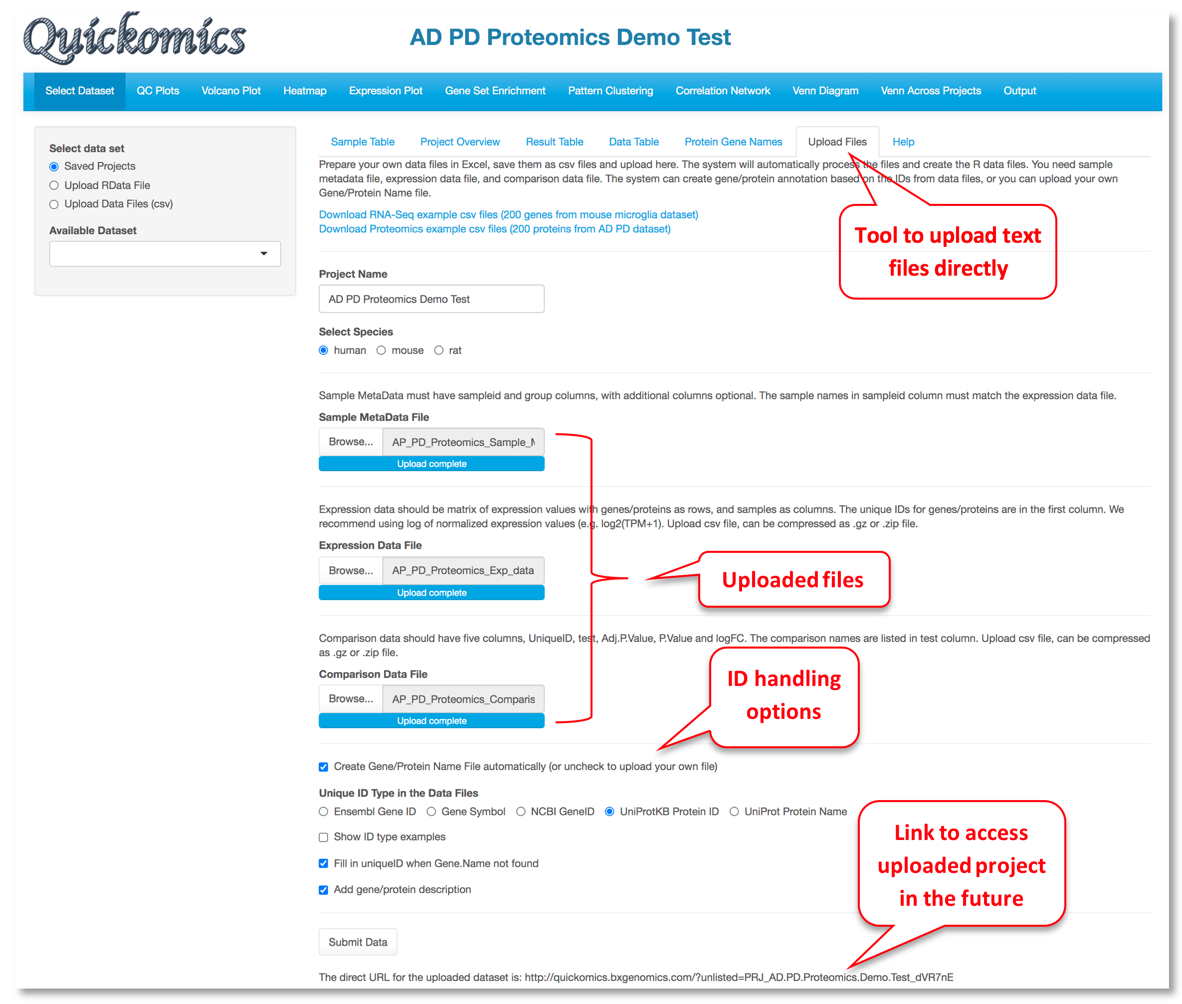
For a data set, the "Upload Files" tool allows users to upload three required files, namely sample metadata, normalized expression data and statistical comparison results in csv format (Comma Separated Values) to Quickomics directly. Example data sets are provided in GitHub for both RNAseq (https://bit.ly/2MRkFcb) and proteomics (https://bit.ly/3rn4i6a). Detailed formatting guidance is outlined below,
- Sample Metadata File: It should have “sampleid” and “group” columns, with additional columns optional. Sample identifiers must match those used in the expression data file.
- Expression Data File: It should be a matrix of expression values with genes/proteins as rows, and samples as columns. The unique IDs for genes/proteins are in the first column. We recommend using log of normalized expression values, e.g. log2(TPM+1) for RNAseq data or normalized intensity or ratio for proteomics data.
- Comparison Data File: It should have five columns, “UniqueID”, “test”, “Adj.P.Value”, “P.Value” and “logFC”. The comparison names are listed in “test” column. Please note that wrongly named column headers will cause issues.
- Optional Gene/Protein Name File: The system has built-in function to convert unique IDs in the data files to gene symbols and create the Gene/Protein Name file, so most users don't need to prepare the file. Nevertheless, if provided by users, it must have four columns: “id” (sequential numbers like 1,2,3 … …), “UniqueID” (matching IDs used in the expression and comparison data file), “Gene.Name” (official gene symbols), “Protein.ID” (UniProt protein IDs, or keep it empty for RNA-Seq data). Additional columns (e.g. gene biotype) are optional.
After the data files are processed, Quickomics will automatically load all required data for exploration immediately and provide a link for the user to come back in the future.
Behind the scene, Bioconductor biomaRt package (https://bioconductor.org/packages/release/bioc/html/biomaRt.html) has been used to convert gene IDs (Ensembl gene, NCBI gene ID, etc.) into gene symbols by querying Ensembl databases. For protein IDs, we generated a custom lookup table using information downloaded from UniProt Knowledgebase to convert UniProt IDs to gene symbols and protein names. We didn't use biomaRt for proteins as Ensembl databases only cover about 60-80% protein IDs in a typical proteomics data set.
We recommend uploading csv files, which is convenient for general users. Nevertheless, experienced R programmers can create R data files to be uploaded through “Upload RData File” option.
Two R data files are required for each data set, one contains the main data and the other contains gene co-expression network information. For the pre-loaded datasets, main data files are located in the “data” folder, https://github.com/interactivereport/Quickomics/tree/master/data, and gene co-expression network files are located in the “networkdata” folder, https://github.com/interactivereport/Quickomics/tree/master/networkdata. One can review the content of a R data file (e.g. Mouse_microglia_RNA-Seq.RData) in the “data” folder by loading it into R. The main R data file contains the following R data frame objects.
- MetaData: It must have “sampleid”, “group”, “Order” and “ComparePairs” columns. Additional metadata columns about samples are optional. “sampleid” should match those used in expression data. “group” holds group names of samples. “Order” is ordered group names used on plotting. “ComparePairs” are names of comparisons performed.
- ProteinGeneName: It must have “UniqueID”, “Gene.Name” and “Protein.ID” columns. “UniqueID” matches gene ID in below data_wide and data_long objects. “Gene.Name” should be official gene symbols. “Protein.ID” is UniProt protein IDs, or empty for RNA-Seq data. Additional columns about proteins or genes are optional.
- data_wide: This is the expression matrix in which rows are genes and columns are samples. Samples must match “sampleid” values in MetaData and gene IDs must match “UniqueID” values in ProteinGeneName.
- data_long: Gene expression matrix in long format with four columns, “UniqueID”, “sampleid”, “expr” and “group”. “group” values must match those listed in MetaData.
- results_long: The comparison results in long format with five columns, “UniqueID”, “test”, “Adj.P.Value”, “P.Value” and “logFC”. “UniqueID” matches “UniqueID” in ProteinGeneName. “test” column has the comparison names that must match “ComparePairs” values in MetaData. The other values are typically computed from statistical analysis, but the data headers must be changed to “Adj.P.Value”, “P.Value” and “logFC”.
- data_results: This is a summary table starting with “UniqueID” and “Gene.Name” columns, then the intensity (max or mean expression value from data_wide for each gene), mean and SD expression values for each group, and finally comparison data (comparison name added as prefix of columns). The network data object is computed from “data_wide” expression matrix by using Hmisc R package exemplified by the code snippet below.
cor_res <- Hmisc::rcorr(as.matrix(t(data_wide)))
cormat <- cor_res$r
pmat <- cor_res$P
ut <- upper.tri(cormat)
network <- tibble::tibble (
    from = rownames(cormat)[row(cormat)[ut]],
    to = rownames(cormat)[col(cormat)[ut]],
    cor  = signif(cormat[ut], 2),
    p = signif(pmat[ut], 2),
    direction = as.integer(sign(cormat[ut]))
)We have provided example input files (TPM and count matrix files, sample grouping file, comparison list file) and the R scripts to generate the main data and network R data files at https://github.com/interactivereport/Quickomics/tree/master/demo_files/Example_RNA_Seq_data. Please note that you may need to modify RNA_Seq_raw2quickomics.R to fit your input files.
- rsem_TPM.txt: The TPM matrix. One can also use RPKM matrix if needed.
- rsem_expected_count.txt: The gene count matrix. We used RSEM counts in this case, but gene count results from other methods can be used as well.
- grpID.txt: This file lists the group information for each sample.
- comparison.txt: This list lists the comparisons to perform (group 1 vs group 2 in each row).
The following command will read the above data files, run differential gene expression analysis using DESeq2, and create main and network R data files.
$ Rscript RNA_Seq_raw2quickomics.RWe have provided the example input files (normalized protein expression, comparison data, sample information, protein and gene names) and the R script to generate the main data and network R data files at https://github.com/interactivereport/Quickomics/tree/master/demo_files/Example_Proteomics_data. Please note that you may need to modify Proteomics2Quickomics.R to fit your input files.
- NormalizedExpression.csv: Normalized protein expression (log2 transformed).
- ComparisonData.csv: Comparison results. The statistic values are: logFC, P.Value and Adj.P.Value. This can be created using R packages like limma.
- Sample.csv: Sample information file.
- ProteinID_Symbol.csv: This file lists the proteinIDs and associate gene symbols.
The following command will read the above data files and create main and network R data files.
$ Rscript Proteomics2Quickomics.RMethod 1. Create conda environment from yml file. This is the easiest way to install all packages. Please download the file https://github.com/interactivereport/Quickomics/blob/master/conda_environment/QuickOmics.yml, load your conda, then run:
conda env create -f QuickOmics.yml
#The above command may take a while, then you will have a new conda environment called QuickOmics
Method 2. Install all packages in your current R environment. Depending on your system, you may need to install other required programs. We recommend using the conda environment method whenever possible.
cran_packages=c("shiny", "shinythemes", "shinyjs", "plotly", "reshape2", "tidyverse", "gplots", "ggpubr",
"gridExtra", "ggrepel", "RColorBrewer", "pheatmap", "rgl", "car", "colourpicker", "VennDiagram", "factoextra",
"openxlsx", "visNetwork", "cowplot", "circlize", "svglite", "shinyjqui", "Hmisc", "ggrastr",
"ggExtra", "networkD3", "vctrs", "ragg", "textshaping", "stringi", "plyr", "png", "psych", "broom")
#Note: Hmisc is not required to run the Shiny app but is needed to prepare network data from expression matrix.
install.packages(cran_packages, repos="http://cran.r-project.org/")  #choose repos based on your location if needed
if (!requireNamespace("BiocManager", quietly = TRUE))
    install.packages("BiocManager")
BiocManager::install(c("Mfuzz", "biomaRt", "ComplexHeatmap", "pathview"))
#Requirements: shiny >= v1.4.0.2 git clone https://github.com/interactivereport/Quickomics.git
Check the following web links on various options to launch the app.
QuickOmics has a feature to load a project directly from URL in the form of https://quickomics.bxgenomics.com/?serverfile=SRP199678, which requires saving project data files to a user-specified directory on the sever hosting QuickOmics. To use this feature, create a file called config.csv in the QuickOmics App folder.
category,value
server_dir,{Path/to/Server/File}
test_dir,{Path/to/Test/Files}
Files stored in server_dir can be loaded by URLs like: https://quickomics.bxgenomics.com/?serverfile=project_ID
Files stored in test_dir can be loaded by URLs like: https://quickomics.bxgenomics.com/?testfile=project_ID
To prepare project files to be loaded via URL, do the following. For each project, besides the two RData files (ProjectID.RData and ProjectID_netword.RData), prepare a ProjectID.csv file with six columns, e.g.
"Name","ShortName","ProjectID","Species","ExpressionUnit","Path"
"RNAseq analysis of sorted microglia","SRP199678","SRP199678","mouse","log2(TPM+0.25)","/camhpc/home/ysun4/RNASequest/example/SRP199678/EA20220329_0"
The last two columns in the csv file are optional but recommended.
Now copy the three files (projectID.RData, ProjectID_netword.RData and ProjectID.csv) inside the server_dir folder as specified by the config.csv file, and the project can be loaded as https://quickomics.bxgenomics.com/?serverfile=project_ID (replace quickomics.bxgenomics.com by the URL of your own QuickOmics instance).

