Library of Algorithms, Data Structures, variety of solutions to common CS problems.
Add this line to your application as managed dependency:
py-algorithms>=0,<1Or install it globally/locally using pip package manager:
$ pip install py-algorithms - Deque
- Stack (LIFO)
- Queue (FIFO)
- Fibonacci Heap (https://en.wikipedia.org/wiki/Fibonacci_heap)
- Min Heap
- Max Heap
- Priority Queue (Fibonacci)
- Min PQ
- Max PQ
- Suffix Array
- Binary Search
  - Quick Sort
  - Shell Sort (Shell method)
  - Heap Sort (Fibonacci heap)
  - Merge Sort
  - Comb Sort
  - Bubble Sort
  - Selection Sort
  - Depth-First-Search (DFS)
  - Breadth-First-Search (BFS)
  - Topologial sort
  - Floyd–Warshall algorithm
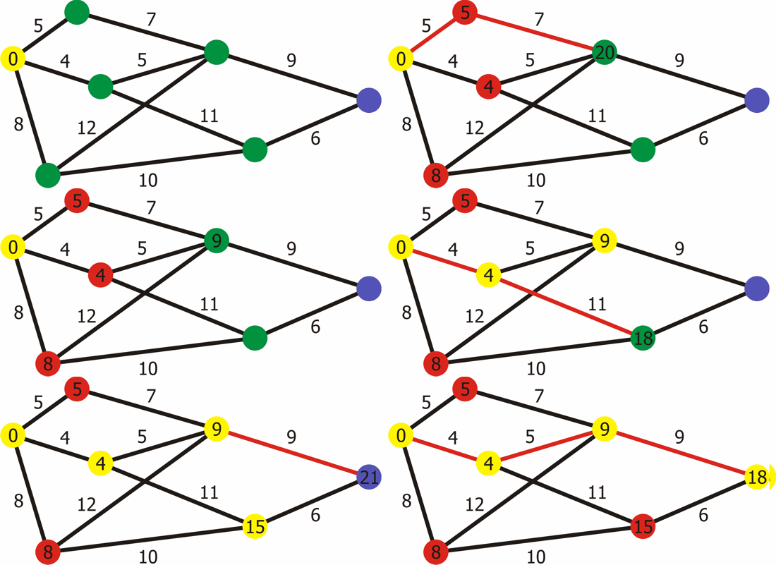
  - Dijkstra's algorithm
  - Patttern Matching
  - Boyer–Moore string search
  - Knut-Morris-Prat string search
  - Miller-Rabin primality test
  - Simple primality test
  - Quick Union
  - Union Find
  - Weighted Union Find
  - Weighted Union Find with Path Compression
  - Longest Increasing Subsequence (LIS)
  - Levenshtein Distance
  - 0-1 Knapsack Problem
  - TopCoder (www.topcoder.com)
  - HackerRank problems & submissions (https://www.hackerrank.com)
  - CoderByte challenges (https://coderbyte.com)
Solutions to specific area problems in Computer Science discipline.
Solutions to various challenges published at https://coderbyte.com
Solutions to various challenges published at https://hackerrank.com
- Binary Search Tree LCA
- Shortest Path in Unweighted Graph with cycles
- Weighted Path
- PowerSet
- Subset Sum
- Two Sum
- Array Addition
Check out unit test in order to take usage examples.
Sort algorithms factory methods implementation will follow functional interface. Old school concrete type disclosure available too as well.
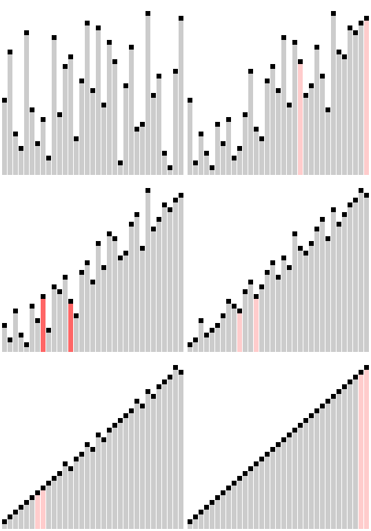
Quicksort (sometimes called partition-exchange sort) is an efficient sorting algorithm, serving as a systematic method for placing the elements of an array in order. Developed by Tony Hoare in 1959 and published in 1961, it is still a commonly used algorithm for sorting. When implemented well, it can be about two or three times faster than its main competitors, merge sort and heapsort.
Worst case: О(n^2)
Best case: О(n log n)
Average: О(n log n)
Space: O(n) naive
from py_algorithms.sort import new_quick_sort

xs = [0, 6, 7, 8, 9, 4, 5, 12, -1]
sorting_algorithm = new_quick_sort()
sorting_algorithm(xs)

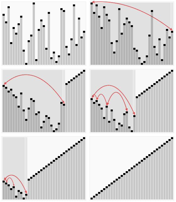
#=> [-1, 0, 4, 5, 6, 7, 8, 9, 12]In computer science, heapsort is a comparison-based sorting algorithm. Heapsort can be thought of as an improved selection sort: like that algorithm, it divides its input into a sorted and an unsorted region, and it iteratively shrinks the unsorted region by extracting the largest element and moving that to the sorted region. The improvement consists of the use of a heap data structure rather than a linear-time search to find the maximum.
Worst case: О(n log n)
Best case: О(n)
Average: О(n log n)
Worst case space: O(1)
from py_algorithms.sort import new_heap_sort

xs = [0, 6, 7, 8, 9, 4, 5, 12, -1]
sorting_algorithm = new_heap_sort()
sorting_algorithm(xs)

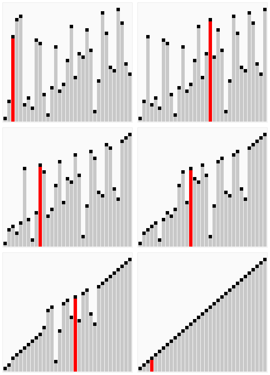
#=> [-1, 0, 4, 5, 6, 7, 8, 9, 12]Shellsort, also known as Shell sort or Shell's method, is an in-place comparison sort. It can be seen as either a generalization of sorting by exchange (bubble sort) or sorting by insertion (insertion sort). The method starts by sorting pairs of elements far apart from each other, then progressively reducing the gap between elements to be compared. Starting with far apart elements, it can move some out-of-place elements into position faster than a simple nearest neighbor exchange. Donald Shell published the first version of this sort in 1959 The running time of Shellsort is heavily dependent on the gap sequence it uses. For many practical variants, determining their time complexity remains an open problem.
Worst case: О(n^2)
Best case: О(n log n)
Average: ~
Worst case space: O(n)
from py_algorithms.sort import new_shell_sort

xs = [0, 6, 7, 8, 9, 4, 5, 12, -1]
sorting_algorithm = new_shell_sort()
sorting_algorithm(xs)

#=> [-1, 0, 4, 5, 6, 7, 8, 9, 12]Bubble sort, sometimes referred to as sinking sort, is a simple sorting algorithm that repeatedly steps through the list to be sorted, compares each pair of adjacent items and swaps them if they are in the wrong order.
Worst case: O(n^2)
Best case: O(n) (if already sorted)
Average: O(n^2)
Worst case space: O(1)
from py_algorithms.sort import new_bubble_sort

sort = new_bubble_sort() # type: Callable[[List[T]], List[T]]
sort([20,15,0,-1,70,-88])

#=> [-88, -1, 0, 15, 20, 70]In computer science, merge sort is an efficient, general-purpose, comparison-based sorting algorithm. Most implementations produce a stable sort, which means that the implementation preserves the input order of equal elements in the sorted output. Mergesort is a divide and conquer algorithm that was invented by John von Neumann in 1945.
Worst case: О(n)
Best case: О(n log n)
Average: О(n log n)
Worst case space: O(n)
from py_algorithms.sort import new_merge_sort

xs = [0, 6, 7, 8, 9, 4, 5, 12, -1]
sorting_algorithm = new_merge_sort()
sorting_algorithm(xs)

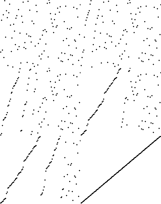
#=> [-1, 0, 4, 5, 6, 7, 8, 9, 12]Comb sort is a relatively simple sorting algorithm originally designed by Włodzimierz Dobosiewicz in 1980. Later it was rediscovered by Stephen Lacey and Richard Box in 1991. Comb sort improves on bubble sort. The basic idea is to eliminate turtles, or small values near the end of the list, since in a bubble sort these slow the sorting down tremendously. Rabbits, large values around the beginning of the list, do not pose a problem in bubble sort.
Worst case: О(n^2)
Best case: О(n log n)
Average: О(n^2)
Worst case space: O(1)
from py_algorithms.sort import new_comb_sort

xs = [0, 6, 7, 8, 9, 4, 5, 12, -1]
sorting_algorithm = new_comb_sort()
sorting_algorithm(xs)

#=> [-1, 0, 4, 5, 6, 7, 8, 9, 12]In computer science, selection sort is a sorting algorithm, specifically an in-place comparison sort. It has O(n^2) time complexity, making it inefficient on large lists, and generally performs worse than the similar insertion sort. Selection sort is noted for its simplicity, and it has performance advantages over more complicated algorithms in certain situations, particularly where auxiliary memory is limited.
Worst case: О(n^2)
Best case: О(n^2)
Average: О(n^2)
Worst case space: O(n)
from py_algorithms.sort import new_selection_sort

xs = [0, 6, 7, 8, 9, 4, 5, 12, -1]
sorting_algorithm = new_selection_sort()
sorting_algorithm(xs)

#=> [-1, 0, 4, 5, 6, 7, 8, 9, 12]In computer science, binary search, also known as half-interval search, logarithmic search, or binary chop, is a search algorithm that finds the position of a target value within a sorted array.
from py_algorithms.search import new_binary_search, Search

array = [0, 4, 5, 6, 7, 8, 9, 12]
algorithm = new_binary_search() # type: Search

algorithm.search(array, 12) #=> 12
algorithm.search(array, 6) #=> 6In computer science, a double-ended queue (dequeue, often abbreviated to deque) is an abstract data type that generalizes a queue, for which elements can be added to or removed from either the front (head) or back (tail)
Deque implementation using doubly-linked list underneath. Operations taking constant time.
from py_algorithms.data_structures import new_deque, Deque

ds = new_deque() # type: Deque
ds.push_back(1)  #=> 1
ds.push_front(2) #=> 2
ds.front         #=> 2
ds.back          #=> 1
ds.pop_front()   #=> 2
ds.size #=> 1FIFO is an acronym for first in, first out, a method for organizing and manipulating a data buffer, where the oldest (first) entry, or 'head' of the queue, is processed first.
from py_algorithms.data_structures import new_queue, Queue

ds = new_queue() # type: Queue
ds.push(1)
ds.push(2)
ds.pop() #=> 1
ds.pop() #=> 2
ds.size #=> 0In computer science, a stack is an abstract data type that serves as a collection of elements, with two principal operations: push, which adds an element to the collection, and pop, which removes the most recently added element that was not yet removed. The order in which elements come off a stack gives rise to its alternative name, LIFO (for last in, first out). Additionally, a peek operation may give access to the top without modifying the stack.
from py_algorithms.data_structures import new_stack, Stack

ds = new_stack() # type: Stack
ds.push(1)
ds.push(2)
ds.pop() #=> 2
ds.pop() #=> 1
ds.size #=> 0In computer science, a Fibonacci heap is a data structure for priority queue operations, consisting of a collection of heap-ordered trees. It has a better amortized running time than many other priority queue data structures including the binary heap and binomial heap. Michael L. Fredman and Robert E. Tarjan developed Fibonacci heaps in 1984 and published them in a scientific journal in 1987. They named Fibonacci heaps after the Fibonacci numbers, which are used in their running time analysis.
*Generic Heap (https://www.cs.princeton.edu/~wayne/teaching/fibonacci-heap.pdf)
Make a new heap with Max property by supplying functor (a: any, b: any) => c: int
from py_algorithms.data_structures import new_heap, Heap

heap = new_heap(lambda x, y: (x > y) - (x < y) == 1) # type: Heap

# Push distinct key value pairs to the heap

heap.push('Kelly', 1)
heap.push('Susan', 8)
heap.push('Ryan', 7)

# Heap should manage to keep highest key & value on the top

heap.next_key #=> 'Susan'
heap.pop()    #=> 8
*MAX Heap (https://en.wikipedia.org/wiki/Min-max_heap)
from py_algorithms.data_structures import new_max_heap, Heap

heap = new_max_heap() # type: Heap

heap.push('Kelly', 1)
heap.push('Susan', 8)
heap.push('Ryan', 7)

# Heap should manage to keep highest key & value on the top

heap.next_key #=> 'Susan'
heap.max      #=> 8
heap.pop()    #=> 8
*MIN Heap (https://en.wikipedia.org/wiki/Min-max_heap)
from py_algorithms.data_structures import new_min_heap, Heap

heap = new_min_heap() # type: Heap

heap.push('One', 1)
heap.push('Eight', -8)
heap.push('Seven', 7)

# Heap should manage to keep lowest key & value on the top

heap.next_key #=> 'Eight'
heap.min      #=> -8
heap.pop()    #=> -8
Priority Queue (https://en.wikipedia.org/wiki/Priority_queue)
In computer science, a priority queue is an abstract data type which is like a regular queue or stack data structure, but where additionally each element has a "priority" associated with it. In a priority queue, an element with high priority is served before an element with low priority. If two elements have the same priority, they are served according to their order in the queue.
Example of a Max PQ data structure
from py_algorithms.data_structures import new_priority_queue

pq = new_priority_queue(lambda x, y: (x > y) - (x < y) == 1)
pq.push('Important', 10)
pq.push('Not So Important', -2)
pq.pop() #=> 'Important'
Suffix Array (https://en.wikipedia.org/wiki/Suffix_array)
In computer science, a suffix array is a sorted array of all suffixes of a string. It is a data structure used, among others, in full text indices, data compression algorithms and within the field of bibliometrics. Suffix arrays were introduced by Manber & Myers (1990) as a simple, space efficient alternative to suffix trees. They have independently been discovered by Gaston Gonnet in 1987 under the name PAT array (Gonnet, Baeza-Yates & Snider 1992).
from py_algorithms.data_structures import new_suffix_array

ds = new_suffix_array('python')
ds.is_sub_str('py') #=> True
ds.is_sub_str('on') #=> True
ds.is_sub_str('ton') #=> True
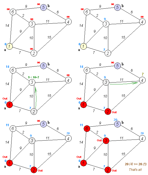
ds.is_sub_str('blah') #=> FalseIn the field of computer science, a topological sort or topological ordering of a directed graph is a linear ordering of its vertices such that for every directed edge uv from vertex u to vertex v, u comes before v in the ordering. For instance, the vertices of the graph may represent tasks to be performed, and the edges may represent constraints that one task must be performed before another; in this application, a topological ordering is just a valid sequence for the tasks. A topological ordering is possible if and only if the graph has no directed cycles, that is, if it is a directed acyclic graph (DAG). Any DAG has at least one topological ordering, and algorithms are known for constructing a topological ordering of any DAG in linear time.
from py_algorithms.graph import new_directed_graph, topological_sort_f1


dag = new_directed_graph()
a = dag.insert_vertex('A')
b = dag.insert_vertex('B')
c = dag.insert_vertex('C')
d = dag.insert_vertex('D')
e = dag.insert_vertex('E')

dag.insert_edge(a, e, None)
dag.insert_edge(b, d, None)
dag.insert_edge(c, d, None)
dag.insert_edge(d, e, None)

topological_sort_f1(dag) #=> [#<Vertex(C)>, #<Vertex(B)>, #<Vertex(D)>, #<Vertex(A)>, #<Vertex(E)>]from py_algorithms.graph import new_undirected_graph
from py_algorithms.graph new_dijkstra_shortest_path
from py_algorithms.graph reconstruct_dijkstra_path_tree
graph = new_undirected_graph()
a = graph.insert_vertex('A')
b = graph.insert_vertex('B')
c = graph.insert_vertex('C')
d = graph.insert_vertex('D')
e = graph.insert_vertex('E')
graph.insert_edge(a, e, 10)
graph.insert_edge(b, d, 2)
graph.insert_edge(c, d, 3)
graph.insert_edge(d, e, 12)
# Start from vertex "c" and grow the cluster.
paths = new_dijkstra_shortest_path(graph, c)
assert paths[c] == 0
assert paths[d] == 3
assert paths[b] == 5
assert paths[e] == 15
assert paths[a] == 25
# Reconstructing all the paths dicovered by algorithm
path_tree = reconstruct_dijkstra_path_tree(graph, c, paths)
# Expanding path from vertex "a" to vertex "c" from "path_tree"
p = a
stack = [a]
while p != c:
p = path_tree[p].opposite(p)
stack.append(p)
assert stack == [a, e, d, c]
# The shortest path to reach vertex "a":
assert stack == [a, e, d, c]In computer science, the Boyer–Moore string search algorithm is an efficient string searching algorithm that is the standard benchmark for practical string search literature. It was developed by Robert S. Boyer and J Strother Moore in 1977. The algorithm preprocesses the string being searched for (the pattern), but not the string being searched in (the text). It is thus well-suited for applications in which the pattern is much shorter than the text or where it persists across multiple searches. The Boyer-Moore algorithm uses information gathered during the preprocess step to skip sections of the text, resulting in a lower constant factor than many other string search algorithms.
from py_algorithms.strings import new_boyer_moore_find

algorithm = new_boyer_moore_find()

substr = 'abcd'
algorithm('foo' + substr + 'bar', substr) # => 3A primality test is an algorithm for determining whether an input number is prime. Among other fields of mathematics, it is used for cryptography. Unlike integer factorization, primality tests do not generally give prime factors, only stating whether the input number is prime or not. Factorization is thought to be a computationally difficult problem, whereas primality testing is comparatively easy (its running time is polynomial in the size of the input). Some primality tests prove that a number is prime, while others like Miller–Rabin prove that a number is composite. Therefore, the latter might be called compositeness tests instead of primality tests.
The Miller–Rabin primality test or Rabin–Miller primality test is a primality test: an algorithm which determines whether a given number is prime, similar to the Fermat primality test and the Solovay–Strassen primality test. Its original version, due to Gary L. Miller, is deterministic, but the correctness relies on the unproven Extended Riemann hypothesis; Michael O. Rabin modified it to obtain an unconditional probabilistic algorithm.
from py_algorithms.primality_tests import new_miller_rabin_primality_test

algorithm = new_miller_rabin_primality_test()

algorithm(199) #=> True, 199 is a prime number
algorithm(4) #=> False, 4 % 2 == 0, therefore, 4 is not a prime number.The test itself is simple and straightforward, but would work very slow on quite big primes.
from py_algorithms.primality_tests import new_simple_primality_test

algorithm = new_simple_primality_test()

algorithm(32416190071) #=> True, 32416190071 is a prime number
algorithm(4) #=> False, 4 % 2 == 0, therefore, 4 is not a prime number.In computer science, mathematics, management science, economics and bioinformatics, dynamic programming (also known as dynamic optimization) is a method for solving a complex problem by breaking it down into a collection of simpler subproblems, solving each of those subproblems just once, and storing their solutions. The next time the same subproblem occurs, instead of recomputing its solution, one simply looks up the previously computed solution, thereby saving computation time at the expense of a (hopefully) modest expenditure in storage space. (Each of the subproblem solutions is indexed in some way, typically based on the values of its input parameters, so as to facilitate its lookup.) The technique of storing solutions to subproblems instead of recomputing them is called "memoization".
In information theory, Linguistics and computer science, the Levenshtein distance is a string metric for measuring the difference between two sequences. Informally, the Levenshtein distance between two words is the minimum number of single-character edits (insertions, deletions or substitutions) required to change one word into the other. It is named after Vladimir Levenshtein, who considered this distance in 1965. Levenshtein distance may also be referred to as edit distance, although that term may also denote a larger family of distance metrics.
It is closely related to pairwise string alignments.
from py_algorithms.strings import new_levenshtein_distance

distance = new_levenshtein_distance(list('Moon'), list("Moore"))
assert 2 == distanceBug reports and pull requests are welcome on GitHub at https://github.com/rlishtaba/py-algorithms. This project is intended to be a safe, welcoming space for collaboration, and contributors are expected to adhere to the Contributor Covenant code of conduct.
The library is available as open source under the terms of the MIT License.
