Stochastic Trajectory Prediction using LSTMs

Author: Todor Davchev, The University of Edinburgh.

Code for the series of blog posts: Colab Link. Some parts of it can be found in Bulgarian at Dev.bg.

It is the building blocks code to Learning Structured Representations of Spatial and Interactive Dynamics for Trajectory Prediction in Crowded Scenes and extended repo here.

If you find this code useful, please cite as follows:

@article{davchev2020learning,
  title={Learning Structured Representations of Spatial and Interactive Dynamics for Trajectory Prediction in Crowded Scenes},
  author={Davchev, Todor Bozhinov and Burke, Michael and Ramamoorthy, Subramanian},
  journal={IEEE Robotics and Automation Letters},
  year={2020},
  publisher={IEEE}
}

The aim of the project is to compare different approaches for trajectory generation. It starts with a very basic and rather intuitive model that doesn't work too well, followed by a simple modification of it that makes all the difference. All future models will build upon the previous ones. The aim is to help the reader gradually build an intuition for trajectory generation.

This repository relies on python 3.6, Tensorflow 1.15.0 and has been tested on an Anaconda environment. Contributions towards extending the platforms and means for running these tutorials along with any suggestions for improvement are highly valued and more than welcome!

Installation

Set up and activate an Anaconda environment, then run the following commands:

git clone git@github.com:tdavchev/stochastic_futures_prediction.git
cd stochastic_futures_prediction
pip install -r requirements.txt
python setup.py install

The code contains a Notebook that has a ready to go code that trains and tests the network. In order to run this, execute:

jupyter notebook

And navigate to Notebooks -> Tutorial 1.ipynb

And -> Tutorial 2.ipynb

Training and Inference

Trainign can be done using relatively small CPU power. The example below training is done using MacBook Pro 13 base model. At train time the output is similar to this:

0/2700 (epoch 0), train_loss = 0.111, time/batch = 0.001
99/2700 (epoch 3), train_loss = 8.332, time/batch = 0.018
198/2700 (epoch 7), train_loss = 0.538, time/batch = 0.015

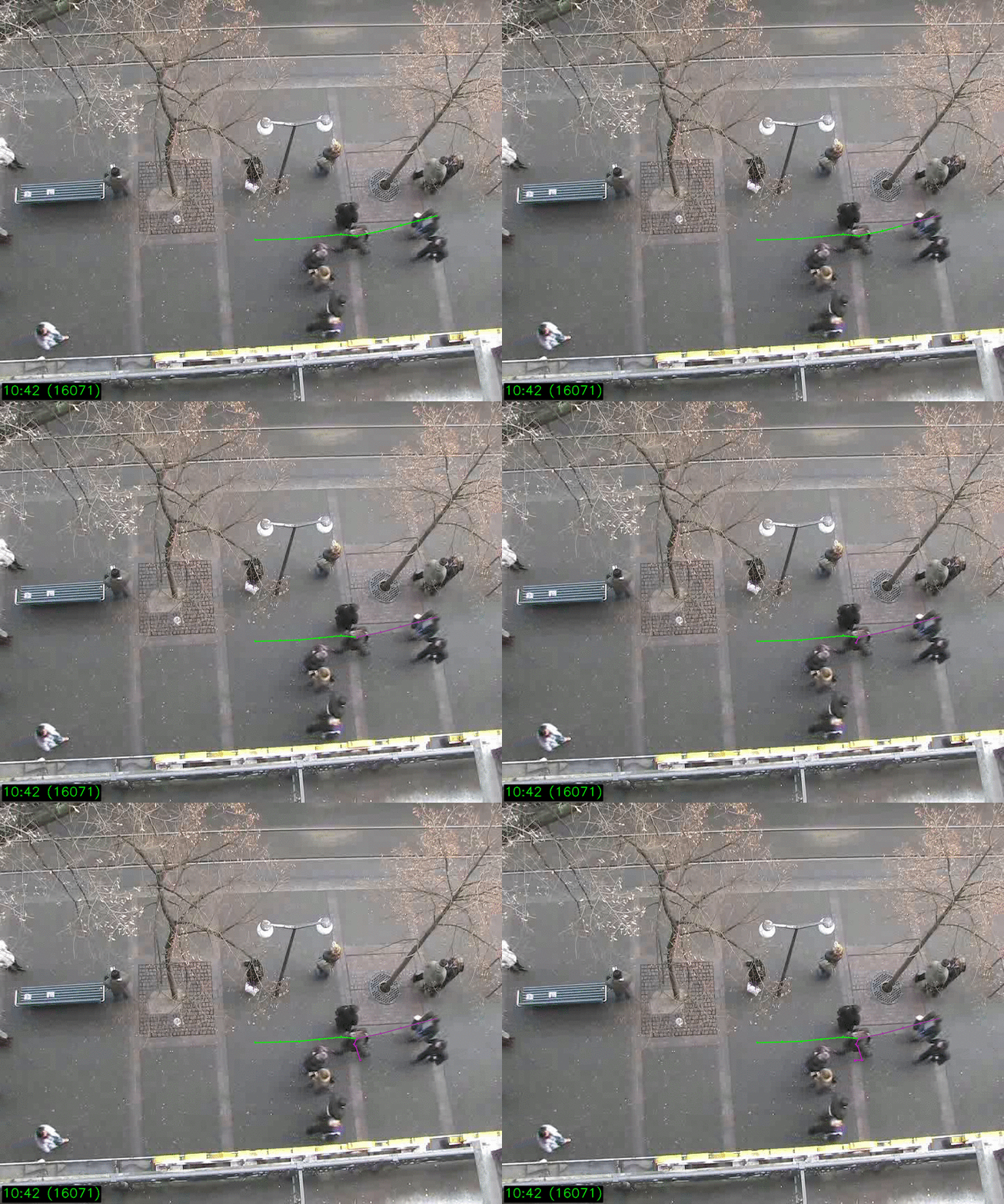
Inference is then done over all trajectories from the test dataset that fit the chosen criteria. Result is obtained from Tutorial 1.

Processed trajectory number :  50 out of  352  trajectories
Processed trajectory number :  100 out of  352  trajectories
Processed trajectory number :  150 out of  352  trajectories
Processed trajectory number :  200 out of  352  trajectories
Processed trajectory number :  250 out of  352  trajectories
Processed trajectory number :  300 out of  352  trajectories
Processed trajectory number :  350 out of  352  trajectories
Total mean error of the model is  0.10521254192652005

Results in:

Project Structure

Project File Structure:
-data
---eth/
------univ/
---------annotated.svg
---------getPixelCoordinates
---------obs_map.pkl
---------pixel_pos_interpolate.csv
---------pixel_pos.csv
---seq_hotel/
------destinations.txt
------groups.txt
------H.txt
------info.txt
------map.png
------obsmat.txt
------README.txt
------seq_hotel.avi
---ucy/
------zara/
---------zara01/
------------annotted.svg
------------getPixelCoordinates.m
------------obs_map.pkl
------------pixel_pos_interpolate.csv
------------pixel_pos.csv
---------zara02/
------------annotted.svg
------------getPixelCoordinates.m
------------obs_map.pkl
------------pixel_pos_interpolate.csv
------------pixel_pos.csv
-notebooks/
---Tutorial 1.ipynb
---Tutorial 2.ipynb
-models
---lstm.py
-utils
---data_tools.py
---distributions.py
---visualisation.py
-setup.py
-requirements.txt
-README.md
-LICENSE

Credits

A massive thank you to the team at Dev.bg for providing me with this incredible opportunity!

Special thanks to J. Geary, D. Angelov, M. Asenov and H. Velev for providing very useful insight about the writing style and clarity of expression for the tutorial and to A. Vemula for providing the Matlab scripts for annotating UCY and ETH University dat sets. This has helped me reduce the time required for setting up this tutorial and provide a comprehensive means to communicate the ideas behind this code.