3. Feature Extraction

General

There are two stages in the audio feature extraction methodology:

• Short-term feature extraction: this is implemented in function feature_extraction() of the ShortTermFeatures.py file. It splits the input signal into short-term widnows (frames) and computes a number of features for each frame. This process leads to a sequence of short-term feature vectors for the whole signal.
• Mid-term feature extraction: In many cases, the signal is represented by statistics on the extracted short-term feature sequences described above. Towards this end, function mid_feature_extraction() from the MidTermFeatures.py file extracts a number of statistcs (e.g. mean and standard deviation) over each short-term feature sequence.

The total number of short-term features implemented in pyAudioAnalysis is 34. In addition, the delta features are optionally computed (they are by default enabled, but can be disabled by setting the deltas argument in feature_extraction() to false). So, the total number of short-term features, including the deltas is 64.

In the following table the complete list of the 34 implemented features is presented:

Feature ID	Feature Name	Description
1	Zero Crossing Rate	The rate of sign-changes of the signal during the duration of a particular frame.
2	Energy	The sum of squares of the signal values, normalized by the respective frame length.
3	Entropy of Energy	The entropy of sub-frames' normalized energies. It can be interpreted as a measure of abrupt changes.
4	Spectral Centroid	The center of gravity of the spectrum.
5	Spectral Spread	The second central moment of the spectrum.
6	Spectral Entropy	Entropy of the normalized spectral energies for a set of sub-frames.
7	Spectral Flux	The squared difference between the normalized magnitudes of the spectra of the two successive frames.
8	Spectral Rolloff	The frequency below which 90% of the magnitude distribution of the spectrum is concentrated.
9-21	MFCCs	Mel Frequency Cepstral Coefficients form a cepstral representation where the frequency bands are not linear but distributed according to the mel-scale.
22-33	Chroma Vector	A 12-element representation of the spectral energy where the bins represent the 12 equal-tempered pitch classes of western-type music (semitone spacing).
34	Chroma Deviation	The standard deviation of the 12 chroma coefficients.

The following code uses feature_extraction() of the ShortTermFeatures.py file to extract the short term feature sequences for an audio signal, using a frame size of 50 msecs and a frame step of 25 msecs (50% overlap). In order to read the audio samples, we call function readAudioFile() from the audioBasicIO.py file.

from pyAudioAnalysis import audioBasicIO
from pyAudioAnalysis import ShortTermFeatures
import matplotlib.pyplot as plt
[Fs, x] = audioBasicIO.read_audio_file("sample.wav")
F, f_names = ShortTermFeatures.feature_extraction(x, Fs, 0.050*Fs, 0.025*Fs)
plt.subplot(2,1,1); plt.plot(F[0,:]); plt.xlabel('Frame no'); plt.ylabel(f_names[0]) 
plt.subplot(2,1,2); plt.plot(F[1,:]); plt.xlabel('Frame no'); plt.ylabel(f_names[1]); plt.show()

Also the code plots the feature sequences of the first two features, i.e. the zero crossing rate and the signal energy. feature_extraction() returns a numpy matrix of 34 rows and N columns, where N is the number of short-term frames that fit into the input audio recording.

Single-file feature extraction - storing to file

The function used to generate short-term and mid-term features is mid_feature_extraction() from the MidTermFeatures.py file. This wrapping functionality also includes storing to CSV files and NUMPY files the short-term and mid-term feature matrices. The command-line way to call this functionality is presented in the following example:

python3 audioAnalysis.py featureExtractionFile -i data/speech_music_sample.wav -mw 1.0 -ms 1.0 -sw 0.050 -ss 0.050 -o data/speech_music_sample.wav

The result of this procedure are two comma-seperated files: speech_music_sample.wav.csv for the mid-term features and speech_music_sample.wav_st.csv for the short-term features. In each case, each feature sequence is stored in a seperate column, in other words, colums correspond to features and rows to time windows (short or long-term). Also, note that for the mid-term feature matrix, the number of features (columns) is two times higher than for the short-term analysis: this is due to the fact that the mid-term features are actually two statistics of the short-term features, namely the average value and the standard deviation. Also, note that in the mid-term feature matrix the first half of the values (in each time window) correspond to the average value, while the second half to the standard deviation of the respective short-term feature. In the same way, the two feature matrices are stored in two numpy files (in this case: speech_music_sample.wav.npy and speech_music_sample.wav_st.npy). So in total four files are created during this process: two for mid-term features and two for short-term features.

Feature extraction - storing to file for a sequence of WAV files stored in a given path

This functionality is the same as the one described above, however it works in a batch mode, i.e. it extracts four feature files for each WAV stored in the given folder. Command-line example:

python3 audioAnalysis.py featureExtractionDir -i data/ -mw 1.0 -ms 1.0 -sw 0.050 -ss 0.050

The result of the above function is to generate feature files (2 CSVs and 2 NUMPY as described above), for each WAV file in the data folder.

Note: the feature extraction process described in the last two paragraphs, does not perform long-term averaging on the feature sequences, therefore a feature matrix is computed for each file (not a single feature vector). See functions directory_feature_extraction() and multiple_directory_feature_extraction() for long-term averaging after the feature extraction process.

Spectrogram and Chromagram visualization

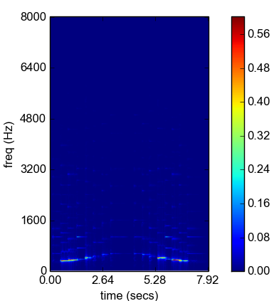
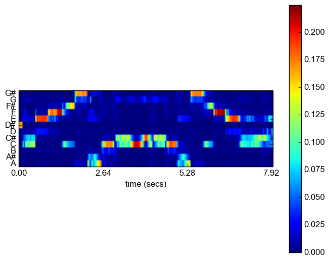
Functions spectrogram() and chromagram() from the ShortTermFeatures.py file can be used to generate the spectrogram and chromagram of an audio signal respectively.

The following command-line example shows how to extract a spectrogram that corresponds to the signal stored in a WAV file:

python audioAnalysis.py fileSpectrogram -i data/doremi.wav

The above command results in the following:

The chromagram is a chroma-time representation, similar to the spectrogram. The following command computes the chromagram of a signal stored in a WAV file:

python audioAnalysis.py fileChromagram -i data/doremi.wav

The above command results in the following:

Beat extraction

Tempo induction is a rather important task in music information retrieval. This library provides a baseline method for estimating the beats per minute (BPM) rate of a music signal. The beat rate estimation is implemented in function beat_extraction() of MidTermFeatures.py file. It accepts 2 arguments: (a) the short-term feature matrix and (b) the window step (in seconds). Obviously, the feature_extraction() function of the ShortTermFeatures.py file is needed to extract the sequence of feature vectors before extracting the beat.

Command-line example:

python audioAnalysis.py beatExtraction -i data/beat/small.wav --plot

The last flag (--plot) enables the visualization of the intermediate algorithmic stages (e.g. feature-specific local maxima detection, etc). Note that visualization can be very time consuming for >1 min signals.

Note that the BPM feature is only applicable in the long-term analysis approach. Therefore, functions that perform long-term averaging on mid-term statistics (e.g. directory_feature_extraction()) have also the choise to compute the BPM (and its confidence value) as features in the long-term feature representation.