Tutorials

Here we provide practical walkthroughs for using factgenie on a specific use-case. For general documentation, please refer to other guides in this wiki.

Note

We assume that you already managed to install and run factgenie. If not, first follow the instructions in Setup and return here later.

Our running example will be the the dataset from Shared Task in Evaluating Semantic Accuracy, which contains statistics from basketball games and model-generated basketball reports:

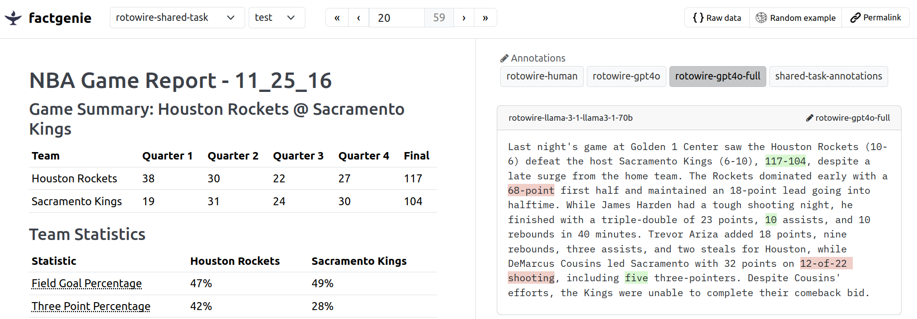
In the tutorials, you will learn the following:

Title	Description
🏀 Tutorial #1: Importing a custom dataset	Loading the basketball statistics and model-generated basketball reports into the web interface.
💬 Tutorial #2: Generating outputs	Using Llama 3.1 with Ollama for generating basketball reports.
📊 Tutorial #3: Customizing data visualization	Creating a custom dataset class for visualizing basketball statistics.
🤖 Tutorial #4: Annotating outputs with an LLM	Using GPT-4o for annotating errors in the basketball reports.
👨‍💼 Tutorial #5: Annotating outputs with human annotators	Using human annotators for annotating errors in the basketball reports.

🏀 Tutorial #1: Importing a custom dataset

The files that we need from the dataset are:

shared_task.jsonl containing inputs and gold reports,
games.csv containing model-generated reports.

These files cannot be yet directly imported into factgenie, but their preprocessing is quite simple.

For starters, we will use one of the pre-defined loaders for importing the dataset.

Specifically, that means:

We will create a JSONL file with the dataset.
We will create a plain text file with the outputs.

Preprocessing data

First, let's download our example data:

# inputs and gold reports
wget "https://raw.githubusercontent.com/ehudreiter/accuracySharedTask/refs/heads/main/shared_task.jsonl"

# model-generated reports
wget "https://raw.githubusercontent.com/ehudreiter/accuracySharedTask/refs/heads/main/games.csv"

Now let's preprocess it into a format that we can load into factgenie

We can do this with the following code extracting the inputs and outputs into separate Python lists:

import pandas as pd
import json

inputs = []
outputs_models = []
outputs_gold = []

# load the model outputs
games_csv = pd.read_csv('games.csv')

# collect the inputs, model outputs and gold outputs
with open('shared_task.jsonl', 'r') as f:
    for line, game in zip(f, games_csv.iterrows()):
        j = json.loads(line)

        outputs_models.append(game[1]['GENERATED_TEXT'])
        outputs_gold.append(j['cleaned_text'])

        # remove any outputs from the input data
        for key in ['cleaned_text', 'detokenized_text', 'summary']:
            j.pop(key)

        inputs.append(j)

The only thing that remains is to save the lists into the respective files:

# save the inputs into a JSONL file
with open('inputs.jsonl', 'w') as f:
    for i in inputs:
        f.write(json.dumps(i) + '\n')

# save the outputs into text files
with open('outputs_gold.txt', 'w') as f:
    for o in outputs_gold:
        f.write(o + '\n')

with open('outputs_model.txt', 'w') as f:
    for o in outputs_models:
        f.write(o + '\n')

That gives us three files: one with the input data (inputs.jsonl) and two files with model outputs (outputs_gold.txt and outputs_model.txt).

We will now upload these files to factgenie through the web interface.

Adding a dataset

To add the dataset into factgenie, we navigate to /manage#external and click on the Add dataset button.

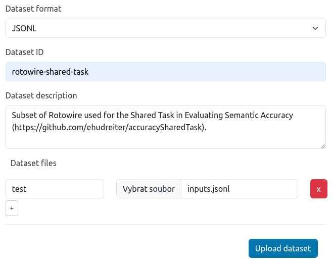
We fill the upload form on the Direct upload tab:

Set the dataset format to JSONL,
Set the dataset name to rotowire-shared-task,
Add the dataset description,
Add a single split called test with our JSONL file.

And click on Upload dataset:

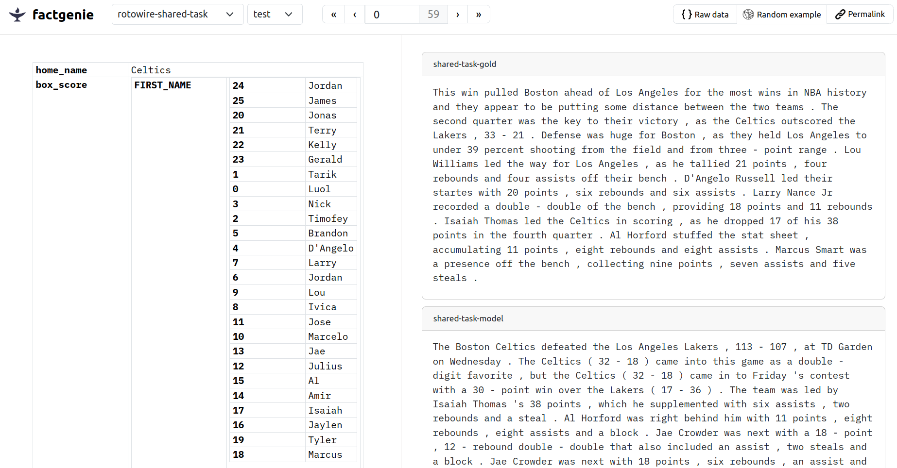
We can now view the inputs in factgenie.

Note

You can see that the JSONL objects are rendered using the json2table package that does decent job at visualizing the data.

We will show how to improve the visualization later in Tutorial #3.

For now, let's also add model outputs.

Adding model outputs

To add the model outputs into factgenie, we navigate to /manage#outputs and click on the Add model outputs button.

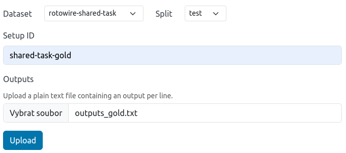
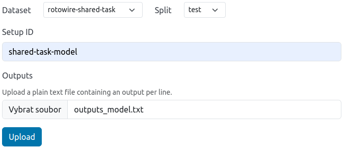
We fill out the form twice, once for every set of outputs (gold and model):

We select the dataset rotowire-shared-task and split test.
We fill in the setup id.
We upload the respective file with the outputs.

After we upload the corresponding files, we can view them in factgenie alongside the inputs.

And that's it! 🎉

Here is our result:

Tip

Our dataset also contains token-level annotations that we can import into factgenie with manual processing. The code is a part of the Jupyter notebook that contains the complete code for this part of the tutorial.

💬 Tutorial #2: Generating outputs

In the previous example, we showed how to import existing model outputs.

Here, we will show how to generate the outputs with our model.

For a more general guide on this, see the section on Generating Outputs.

Setting up an LLM through Ollama

First, we need to decide how we will access the LLM generating the outputs. In this case, we decide to run the model locally.

Specifically, we will run a llama-3.1:70B model with 4-bit quantization through Ollama, an open-source framework for LLM inference.

Note

If you would rather like to see how to use a model through an external API, see 🤖 Tutorial #4 where we use the OpenAI API.

Tip

We also support vLLM vLLM serving instead of ollama. The vLLM may be harder to setup and requires a GPU. However, vLLM supports structured generation via the --guided_json schema specification.. Structured decoding means no parsing errors even for weaker models 🎉.

We follow the installation instructions, which you can find here. For Linux, it involves either running an installation script, or – if we rather do install packages manually – downloading a tarball and unpacking it.

Our next steps are:

running ollama: ollama serve,
downloading the model: ollama pull llama3.1:70b (you only need to do that once),
loading the model: ollama run llama3.1:70b.

Tip

The steps may have changed in the meantime. Always refer to the up-to-date documentation of the framework.

From now on, we assume that the model API is accessible at http://localhost:11434/api/.

Starting a campaign

We will use the page Generate with LLMs and set up a new campaign there. Generation page

After we choose the campaign id and click Next, we get to the main configuration screen.

Here are the options we configured in the web interface (for the sake of brevity shown in the form of the exported YAML config):

type: ollama_gen
model: llama3.1:70b
prompt_template: |-
  Given the JSON-structured data about a basketball game:
  ```
  {data}
  ```
  Generate a one-paragraph basketball summary in natural language.

  Make sure that your report is firmly grounded in the provided data.
system_msg: You are an expert automatic data reporting system.
start_with: |-
  Sure, here is the summary:
  "
api_url: http://localhost:11434/api/
model_args:
  num_ctx: '16384'
  num_predict: '1024'
  seed: '42'
  temperature: '1.0'
  top_k: '50'
  top_p: '0.9'
extra_args:
  remove_suffix: '"'

Comments:

Our prompt contains the placeholder {data}. Factgenie will replace this placeholder with the input data for each example.
We use the parameter start_with. It allows us to slip a prefix that the model "started" its answer with. The model should now start generating the report straight away, without any extra comments. It should also denote the end the report with another quote.
The extra_args field are the arguments that are passed to the model class in factgenie. In this case, we use the remove_suffix argument that the model class recognizes. We use it to remove the closing quote.
We pass the model several arguments which control the generation process. Note especially the num_ctx: 16384 parameter which enlarges the size of the input context window . By default, the size is set to 2048, which would be too short to fit our inputs.

Running a campaign

To run the generated campaign, we click on the campaign name:

and select "Run generation":

As soon as the LLM starts generating outputs, we can see the outputs in the respective rows:

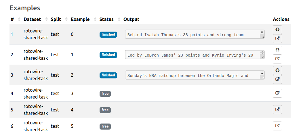
The outputs are not yet available on the Browse page. To make them available, we first need use the Save as model outputs feature on the detail page 👇️

Once we do that, we can see our generated outputs alongside each example 💪

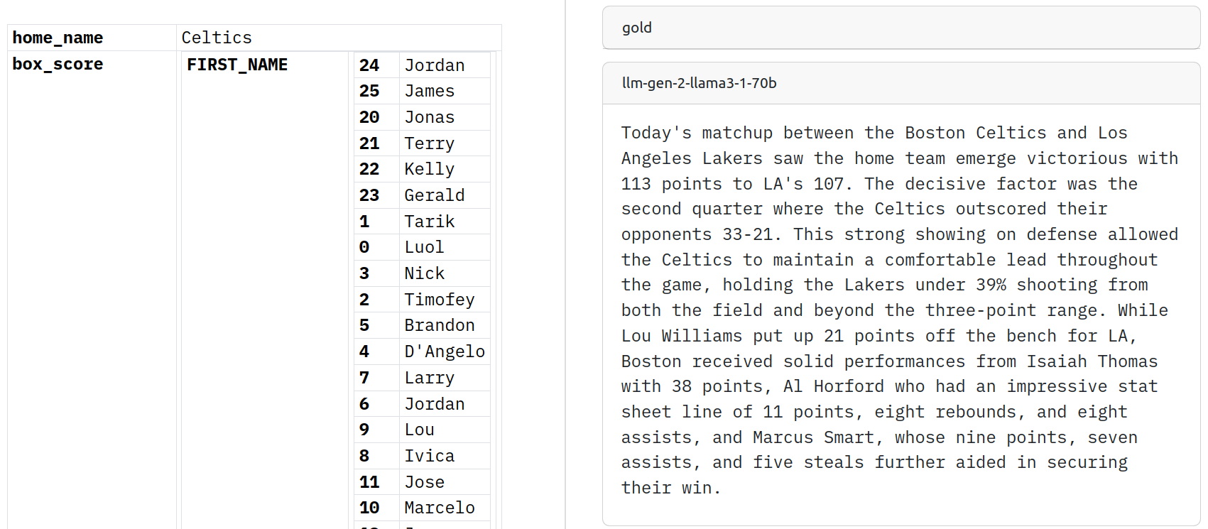
📊 Tutorial #3: Customizing data visualization

You may have noticed that our data representation is not great. Our raw data does not fit the model context size and the tables look a bit disordered.

In this part, we will define a custom data loader that will help us solve these issues.

Important

To follow this part of the tutorial, you need to be able to access the factgenie source files. Make sure that you have installed factgenie as an editable package.

Creating a custom dataset loader

First, we go to factgenie/data/datasets.yml and change the class name:

rotowire-shared-task:
  class: rotowire_shared_task.RotowireSharedTask

That tells us that our dataset is loaded with a class RotowireSharedTask in factgenie/datasets/rotowire_shared_task.py. We will now proceed to implement this class.

Our class will implement two methods: load_examples(split, data_path) and render(example).

The idea is that we will:

Transform each JSONL object into a set of Markdown tables, serving us as a compact model input.
Render the Markdown tables in HTML, serving us as input visualization for annotators and app users.

Representing examples as Markdown tables

We create a file factgenie/datasets/rotowire_shared_task.py with the following content:

from factgenie.datasets.dataset import Dataset
import json

class RotowireSharedTask(Dataset):
  def load_examples(self, split, data_path):
      examples = []

      with open(f"{data_path}/{split}.jsonl") as f:
          lines = f.readlines()
          for line in lines:
              j = json.loads(line)
              summary = self.json_to_markdown_tables(data=j)
              examples.append(summary)

      return examples

The method iterates over the JSONL file and represents each example as a string. The string contains a set of Markdown tables with the game statistics.

The only thing we now need to implement is the self.json_to_markdown_tables(data) method that creates the Markdown table representation.

To make our life easier, we consulted an LLM and it came up with the following tranformations:

import textwrap

def create_game_summary_table(self, data):
    home_team = f"{data['home_city']} {data['home_name']}"
    away_team = f"{data['vis_city']} {data['vis_name']}"

    summary_table = textwrap.dedent(
        f"""\
        #### Game Summary: {away_team} @ {home_team}
        | Team        | Quarter 1                            | Quarter 2                            | Quarter 3                            | Quarter 4                            | Final                           |
        | ----------- | ------------------------------------ | ------------------------------------ | ------------------------------------ | ------------------------------------ | ------------------------------- |
        | {away_team} | {data['vis_line']['TEAM-PTS_QTR1']}  | {data['vis_line']['TEAM-PTS_QTR2']}  | {data['vis_line']['TEAM-PTS_QTR3']}  | {data['vis_line']['TEAM-PTS_QTR4']}  | {data['vis_line']['TEAM-PTS']}  |
        | {home_team} | {data['home_line']['TEAM-PTS_QTR1']} | {data['home_line']['TEAM-PTS_QTR2']} | {data['home_line']['TEAM-PTS_QTR3']} | {data['home_line']['TEAM-PTS_QTR4']} | {data['home_line']['TEAM-PTS']} |
    """
    )
    return summary_table

def create_team_stats_table(self, data):
    home_team = f"{data['home_city']} {data['home_name']}"
    away_team = f"{data['vis_city']} {data['vis_name']}"

    team_stats_table = textwrap.dedent(
        f"""\
        #### Team Statistics
        | Statistic              | {away_team}                         | {home_team}                          |
        | ---------------------- | ----------------------------------- | ------------------------------------ |
        | Field Goal Percentage  | {data['vis_line']['TEAM-FG_PCT']}%  | {data['home_line']['TEAM-FG_PCT']}%  |
        | Three Point Percentage | {data['vis_line']['TEAM-FG3_PCT']}% | {data['home_line']['TEAM-FG3_PCT']}% |
        | Free Throw Percentage  | {data['vis_line']['TEAM-FT_PCT']}%  | {data['home_line']['TEAM-FT_PCT']}%  |
        | Rebounds               | {data['vis_line']['TEAM-REB']}      | {data['home_line']['TEAM-REB']}      |
        | Assists                | {data['vis_line']['TEAM-AST']}      | {data['home_line']['TEAM-AST']}      |
        | Turnovers              | {data['vis_line']['TEAM-TOV']}      | {data['home_line']['TEAM-TOV']}      |
    """
    )
    return team_stats_table

def create_player_stats_tables(self, data):
    def create_single_team_table(team_city, box_score):
        table = textwrap.dedent(
            f"""\
            #### {team_city} Player Statistics
            | Player | Minutes | Points | Rebounds | Assists | Field Goals | Three Pointers | Free Throws | Steals | Blocks | Turnovers |
            | ------ | ------- | ------ | -------- | ------- | ----------- | -------------- | ----------- | ------ | ------ | --------- |\n"""
        )

        for pid in box_score["PLAYER_NAME"].keys():
            if box_score["TEAM_CITY"][pid] == team_city and box_score["MIN"][pid] != "N/A":

                name = f"{box_score['FIRST_NAME'][pid]} {box_score['SECOND_NAME'][pid]}"
                fg = f"{box_score['FGM'][pid]}/{box_score['FGA'][pid]}"
                tpt = f"{box_score['FG3M'][pid]}/{box_score['FG3A'][pid]}"
                ft = f"{box_score['FTM'][pid]}/{box_score['FTA'][pid]}"

                table += f"| {name} | {box_score['MIN'][pid]} | {box_score['PTS'][pid]} | "
                table += f"{box_score['REB'][pid]} | {box_score['AST'][pid]} | "
                table += f"{fg} | {tpt} | {ft} | "
                table += f"{box_score['STL'][pid]} | {box_score['BLK'][pid]} | {box_score['TO'][pid]} |\n"

        return table

    home_table = create_single_team_table(data["home_city"], data["box_score"])
    away_table = create_single_team_table(data["vis_city"], data["box_score"])

    return f"{home_table}\n{away_table}"

We can now use these methods for the json_to_markdown_tables() method:

def json_to_markdown_tables(self, data):
    markdown = f"## NBA Game Report - {data['day']}\n\n"
    markdown += self.create_game_summary_table(data)
    markdown += "\n"
    markdown += self.create_team_stats_table(data)
    markdown += "\n"
    markdown += self.create_player_stats_tables(data)
    return markdown

Rendering Markdown in HTML

The second method we need to implement is the render() method.

As an extra step we add here explanations of the abbreviations to make it easier for human annotators to understand the tables:

def add_explanations(self, html):
    abbr_mappings = {
        "Minutes": "The number of minutes played",
        "Points": "Total points scored",
        "Rebounds": "Total rebounds (offensive + defensive)",
        "Assists": "Passes that directly lead to a made basket",
        "Field Goals": "Shows makes/attempts for all shots except free throws",
        "Three Pointers": "Shows makes/attempts for shots beyond the three-point line",
        "Free Throws": "Shows makes/attempts for uncontested shots awarded after a foul",
        "Steals": "Number of times the player took the ball from the opposing team",
        "Blocks": "Number of opponents' shots that were blocked",
        "Turnovers": "Number of times the player lost the ball to the opposing team",
        "Field Goal Percentage": "The percentage of shots made (excluding free throws)",
        "Three Point Percentage": "The percentage of three-point shots made",
        "Free Throw Percentage": "The percentage of free throws made",
    }

    for term, explanation in abbr_mappings.items():
        html = html.replace(term, f'<abbr title="{explanation}">{term}</abbr>')

    return html

Our method render() method is otherwise very simple. It simply uses the Python markdown package to convert the markdown tables to HTML and adds a few Bootstrap classes:

import markdown

def render(self, example):
    html = markdown.markdown(example, extensions=["markdown.extensions.tables"])
    html = html.replace("<table>", '<table class="table table-hover table-sm">')
    html = self.add_explanations(html)

    return html

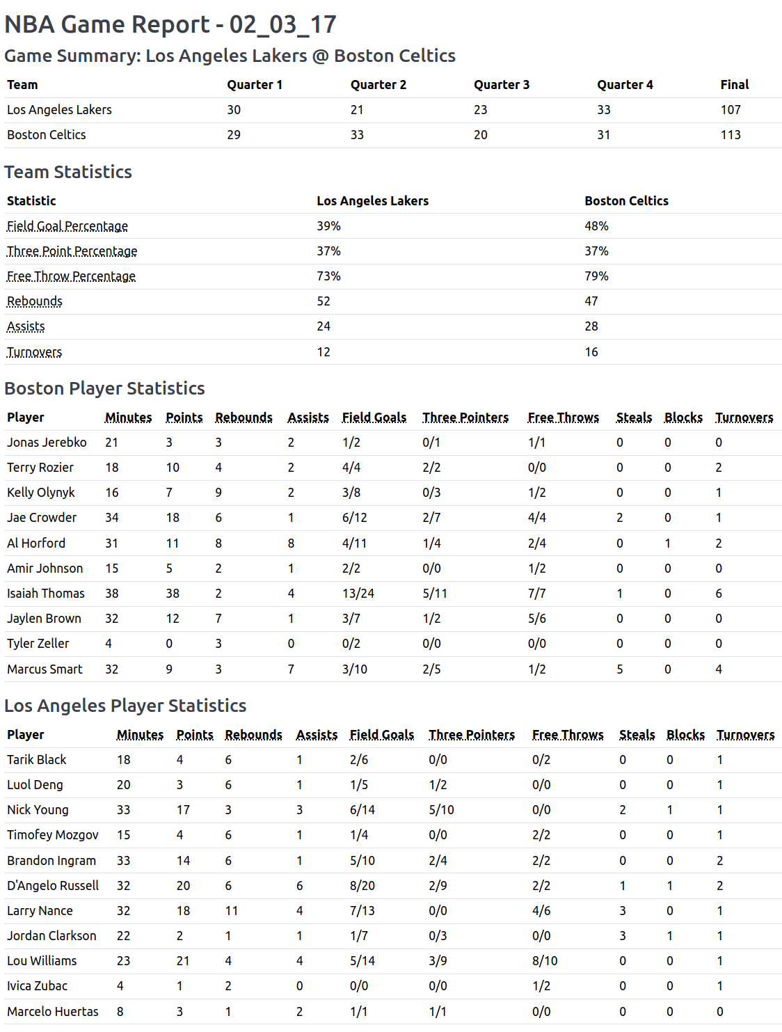
And this is our result. Neat, right? 🤩

Note

We were able to reduce the number of input tokens approximately 3x. Our tables area now also more descriptive and compact.

🤖 Tutorial #4: Annotating outputs with an LLM

Now we can finally get to the core task of factgenie: annotating errors in the generated outputs!

For a more general guide on this, see the section on LLM Annotations.

Setting up GPT-4o

Similarly to the part where we generated the inputs, we need to set up the LLM that we will be accessing.

Here, we will use GPT-4o, one of the recent OpenAI models.

(The reason is that in the case of structured prediction with detailed instructions, proprietary models turn out to be better than the open-source ones. It also allows us to showcase another approach.)

The steps we need to do are the following:

create an OpenAI account,
obtain the API key,
set the API key as an environmental variable before running factgenie:

export OPENAI_API_KEY="<your_key>"

Tip

If you would rather wish to use a local model running through Ollama, see the tutorial on generating outputs where we use OpenAI API.

Starting the campaign

We will use the page Annotate with LLMs and set up a new campaign there.

After we choose the campaign id and click Next, we get to the main configuration screen.

Here are the options we configured in the web interface:

type: openai_metric
system_msg: You are an expert error annotation system. You undestand structured data
  and you can correcly operate with units and numerical values. You are designed to
  output token-level annotations in JSON.
model: gpt-4o-mini-2024-07-18
prompt_template: |-
  [see below for full prompt]
api_url: ''
model_args:
  seed: '42'
  temperature: '0'
annotation_span_categories:
- color: '#d6d0f7'
  name: NUMBER
- color: '#d8f7d0'
  name: NAME
- color: '#f0cfc9'
  name: WORD
- color: '#eacded'
  name: CONTEXT
- color: '#e3cac9'
  name: NOT_CHECKABLE
- color: '#cef3f7'
  name: OTHER
extra_args: {}

Full prompt available here

Comments:

We replicate the instructions for the original shared task to a degree, but we simplified and adapted the instructions for the LLM input.
We give very detailed instructions in the prompt, including the number of each error category and the specific keys that should be included in the output JSON. If the model would not be adhering to these instructions, factgenie would fail to parse the output annotations.
We also include an example of an annotation for a specific example which further helps to guide the model.
While the category colors are arbitrary, the category position is not: the order needs to correspond to the indices specified in the prompt.

On the Data tab, we select our generated outputs for annotation.

Running the campaign

To run the campaign, we click on the campaign name:

and select "Run generation":

As soon as the LLM starts generating outputs, we can see the outputs in the respective rows:

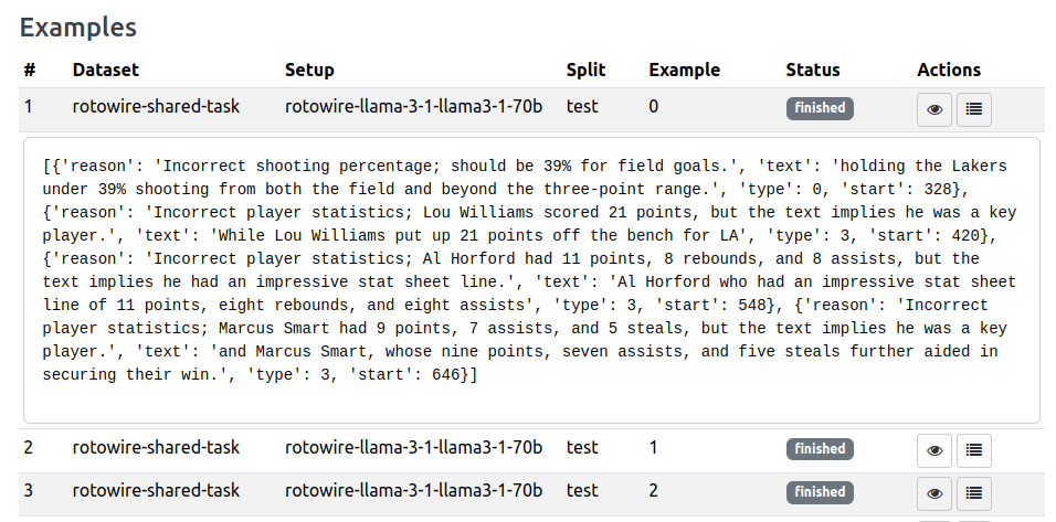
If we click on the 👁️ button, we also get to the Browse interface where we can immediately display our annotations:

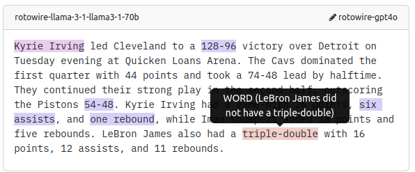
Can you now see how to fit factgenie to your use-case? 😎

👨‍💼 Tutorial #5: Annotating outputs with human annotators

At this point, you may wonder: how would human annotators annotate the same outputs?

To find out, we will also run a human evaluation campaign, using the same data and similar parameters.

For a more general guide on this, see the section on Crowdsourcing Annotations.

Gathering human annotators

In this tutorial, we will stick here with the simplest case in which we personally know the human annotators (perhaps our colleagues or domain experts we hired) and we will share with them the URL of the annotation app manually.

Tip

Factgenie also supports crowdsourcing services, please see the above guide for details.

Starting the campaign

Since we want to replicate the LLM evaluation campaign, we can make our job slightly easier by duplicating our LLM config.

To do that, we:

go to the list of campaigns,
click the menu icon on the row with the campaign,
go to the Duplicate / export tab,
select "Save crowdsourcing config".

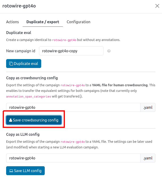
Now we can use the page Annotate with human annotators to set up a new campaign there.

After we choose the campaign id and click Next, we get to the main configuration screen.

Here are the options we configured in the web interface.

annotation_granularity: words
annotation_span_categories:
- color: '#d8f7d0'
  name: NAME
- color: '#d6d0f7'
  name: NUMBER
- color: '#f0cfc9'
  name: WORD
- color: '#e3cac9'
  name: NOT_CHECKABLE
- color: '#eacded'
  name: CONTEXT
- color: '#cef3f7'
  name: OTHER
annotator_instructions: |-
  In this task, you will annotate outputs of an automatic text generation system. For each example, you will see **data** from a basketball game on the left side and the corresponding generated **text** on the right side. Your task is to **annotate errors** in the text with respect to the data.

  There are six types of errors that you can mark in the generated text:

  1. <b><span style="background-color: #d6d0f7">NAME</span></b> (Incorrect named entity): This includes people, places, teams, and days of the week.
  2. <b><span style="background-color: #d8f7d0">NUMBER</span></b> (Incorrect number): It does not matter whether the number is spelled out or is in digits.
  3. <b><span style="background-color: #f0cfc9">WORD</span></b> (Incorrect word): A word which is not one of the above and is incorrect.
  4. <b><span style="background-color: #eacded">NOT_CHECKABLE</span></b> (Not checkable): A statement which can not be checked, either because the information is not available or because it is too time-consuming to check.
  5. <b><span style="background-color: #e3cac9">CONTEXT</span></b> (Context error): A phrase which causes an incorrect inference because of context or discourse.
  6. <b><span style="background-color: #cef3f7">OTHER</span></b> (Other): Any other type of mistake.

  You can annotate the errors by selecting the appropriate error category and dragging your mouse over the text, highlighting the error span.

  Once you think you have marked all the errors present in the text, click the **✅ Mark example as complete** button (you can still update the annotation later).

  You will be able to submit the annotations once they are all are marked as complete.
service: local
examples_per_batch: 5
annotators_per_example: 1
final_message: Your annotations have been submitted.
flags: []
has_display_overlay: true
idle_time: 60
options: []
sort_order: shuffle-all

Comments:

We used the preset rotowire-gpt4o.yaml that we exported from the LLM campaign. This automatically pre-filled the list of annotation span categories.
As we are not comparing outputs from different systems, we selected shuffle_all to give each annotator a random subset of examples.
We adapted the instructions for human annotators.
We do not need to specify completion code in the final message (unlike when using a crowdsourcing service).

Preview the campaign

To make sure we prepared everything correctly, we can view the annotation page using the Preview button:

Here, we see everything that an annotator will see all the way to submitting the annotations.

Note

If you submit the annotations in the preview mode, make sure to delete them manually.

Sharing the campaign with the annotators

On the campaign detail page, we can see the page link, e.g.:

http://localhost:8890/annotate?campaign=rotowire-human&annotatorId=FILL_YOUR_NAME_HERE

This is the URL that we will send to the annotators.

We need to make sure that factgenie is running on an URL accesible to the annotators as well.

We also need to instruct the annotators to replace the FILL_YOUR_NAME_HERE placeholder with their identifier.

Monitoring the annotators

Each annotator is assigned a batch of examples.

Until they submit the annotations (or until the idle_time elapsed), this batch cannot be assigned to any other annotator.

Once an annotator submits the annotations, their batch is marked as finished.

We can monitor the status of each batch on the campaign detail page:

Viewing the results

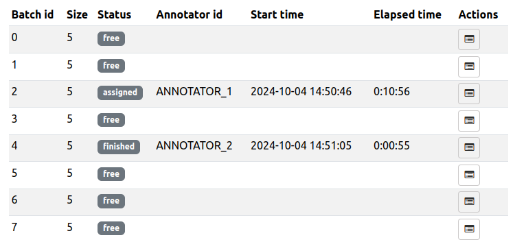
Similarly to the LLM evaluation campaigns, we can immediately view the collected annotations on the Browse page.

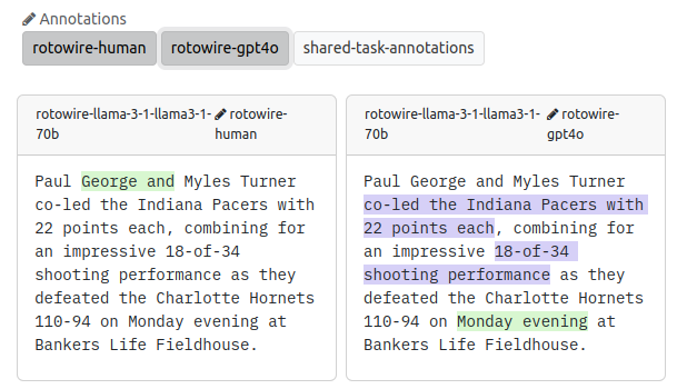
Since we have collected annotations for the same set of outputs, we can now view the results side by side:

We can also use the Analysis page to view statistics of the annotations, which we plan to describe in the next tutorial.

Now go and start annotating with factgenie yourselves! 🌈

Guides

Tutorials

🏀 Importing a custom dataset
💬 Generating outputs
📊 Customizing data visualization
🤖 Annotating outputs with an LLM
👨‍💼 Annotating outputs with human annotators

Provide feedback

Saved searches

Use saved searches to filter your results more quickly

Tutorials

Tutorials

🏀 Tutorial #1: Importing a custom dataset

Preprocessing data

Adding a dataset

Adding model outputs

💬 Tutorial #2: Generating outputs

Setting up an LLM through Ollama

Starting a campaign

Running a campaign

📊 Tutorial #3: Customizing data visualization

Creating a custom dataset loader

Representing examples as Markdown tables

Rendering Markdown in HTML

🤖 Tutorial #4: Annotating outputs with an LLM

Setting up GPT-4o

Starting the campaign

Running the campaign

👨‍💼 Tutorial #5: Annotating outputs with human annotators

Gathering human annotators

Starting the campaign

Preview the campaign

Sharing the campaign with the annotators

Monitoring the annotators

Viewing the results

Guides

Tutorials

Clone this wiki locally