Quick Start of Distributed ZOOpt

Distributed ZOOpt is the distributed version of ZOOpt. In order to improve the efficiency of handling distributed computing, we use Julia language to code the client end for its high efficiency and Python-like features ( ZOOclient ). Meanwhile, the servers are still coded in Python (ZOOsrv) . Therefore, users programs their objective function in Python as usual, and only need to change a few lines of the client Julia codes (just as easy to understand as Python).

Two zeroth-order optimization methods are implemented in Distributed ZOOpt release 0.1, respectively are Asynchronous Sequential RACOS (ASRacos) method and parallel pareto optimization for subset selection method (PPOSS, IJCAI'16)

Installation

Distributed ZOOpt contains two parts: ZOOclient and ZOOsrv. Hence, to use it, users should install ZOOclient and ZOOsrv respectively.

Install ZOOclient

If you have not done so already, download and install Julia (Any version starting with 0.6 should be fine)

To install ZOOclient, start Julia and run:

Pkg.add("ZOOclient")

This will download ZOOclient and all of its dependencies.

Install ZOOsrv

The easiest way to get ZOOsrv is to type pip install zoosrv in you terminal/command line.

If you want to install ZOOsrv by source code, download this project and sequentially run following commands in your terminal/command line.

$ python setup.py build
$ python setup.py install

A Quick Example

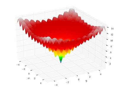
We will demonstrate Distributed ZOOpt by using it to optimize Ackley function.

Ackley function is a classical function with many local minima. In 2-dimension, it looks like (from wikipedia)

1. Define the Ackley function using Python for minimization.

   import numpy as np
   def ackley(solution):
       x = solution.get_x()
       bias = 0.2
       value = -20 * np.exp(-0.2 * np.sqrt(sum([(i - bias) * (i - bias) for i in x]) / len(x))) - \
               np.exp(sum([np.cos(2.0*np.pi*(i-bias)) for i in x]) / len(x)) + 20.0 + np.e
       return value	

2. Start the control server by providing a port.

   from zoosrv import control_server
   
   control_server.start(20000)

3. Start evaluation servers by providing a configuration file.

   from zoosrv import evaluation_server
   
   evaluation_server.start("evaluation_server.cfg")

   configuration file is listed as follows:

   [evaluation server]
   shared fold = /path/to/project/ZOOsrv/example/objective_function/
   control server's ip_port = 192.168.0.103:20000
   evaluation processes = 10
   starting port = 60003
   ending port = 60020
   

   shared fold indicates the root directory your julia client and evaluation servers work under. The objective function should be defined under this directory. constrol server's ip_port means the address of the control server. The last three lines state we want to start 10 evaluation processes by choosing 10 available ports from 60003 to 60020.

4. Write client code using Julia language and run this file.

   client.jl

   using ZOOclient
   using PyPlot
   
   # define a Dimension object
   dim_size = 100
   dim_regs = [[-1, 1] for i = 1:dim_size]
   dim_tys = [true for i = 1:dim_size]
   mydim = Dimension(dim_size, dim_regs, dim_tys)
   # define an Objective object
   obj = Objective(mydim)
   
   # define a Parameter Object, the five parameters are indispensable.
   # budget:  number of calls to the objective function
   # evalueation_server_num: number of evaluation cores user requires
   # control_server_ip_port: the ip:port of the control server
   # objective_file: objective funtion is defined in this file
   # func: name of the objective function
   par = Parameter(budget=10000, evaluation_server_num=10, control_server_ip_port="192.168.1.105:20000",      objective_file="fx.py", func="ackley")
   
   # perform optimization
   sol = zoo_min(obj, par)
   # print the Solution object
   sol_print(sol)
   
   # visualize the optimization progress
   history = get_history_bestsofar(obj)
   plt[:plot](history)
   plt[:savefig]("figure.png")

   To run this file, type the following command

   $ ./julia -p 4 /absolute/path/to/your/file/client.jl
   

   Starting with julia -p n provides n worker processes on the local machine. Generally it makes sense for n to equal the number of CPU cores on the machine.

For a few seconds, the optimization is done and we will get the result.

Visualized optimization progress looks like:

Release 0.1

• Include the asynchronous version of the general optimization method Sequential RACOS (AAAI'17)
• Include the Parallel Pareto Optimization for Subset Selection method (PPOSS, IJCAI'16)

​ ​ ​