-
Notifications
You must be signed in to change notification settings - Fork 17
Building a Canopy Height Model (CHM) using lidR
In theory Canopy Height Models (CHM) can be easily derived from airborne LiDAR data. Since they are rasterized, they can be understood as an aggregated simplification of the underlying 3D point cloud model. CHMs are obviously representing the tree canopy. In addition it should be noted that a reliable CHM should has removed all other above-ground features such as buildings etc.
There are some open source software tools that can deal with LiDAR derived point clouds as creating DTMs and DSMs. Just to name a few examples GRASS GIS, the liblas libraries as well as the Fusion Tools.
You will also find some blogs and course material dealing with the topic. To list just a few most obvious Rasterizing perfect canopy height models which is a lidR clone of Martin Isenburgs Rasterizing Perfect Canopy Height Models from LiDAR. The regular MSC courses at Marburg University are also dealing with the LiDAR topic (e.g. Spotlight LiDAR, gihub repo of 2017 class and more.)
However with respect to comfort, flexibility, big data cpabilities and scalability, open source and integeration to automated workflows the R package lidR package is probably the very best choice.
Nevertheless in practicse using authority provided LiDAR data may yield some massive limitations. What you might not expect in particular corrupt header erroneous spatial referencing and often inefficient classification of the “ground” points are part of everyday life. Despite the high demand to be able to use LiDAR data correctly, there is almost a hype in the user scene, especially in the last few years. While LiDAR data is still demanding in use, it is available to a growing number of users. An essential step towards simplified use is to create rasterized, two-dimensional excerpts of the data and to work with them. Probably the best know are the DTM,DSM and resulting the CHMs which are very useful for all kind of forest and ecological management, for conservation biology and a lot of other topics.
First we have to set up the project. We create a fixed folder structure.
devtools::install_github("gisma/uavRst", ref = "master")
require(raster)
require(mapview)
require(lidR)

# proj subfolders
projRootDir<-tempdir()

#source("src/mpg_course_basic_setup.R")
project_folders = c("data/lidar/level1/",
                    "data/lidar/level1/example/",
                    "data/lidar/level2/")

# create pathes
path<-link2GI::initProj(projRootDir = projRootDir,
                        projFolders = project_folders)

# get some colors
pal = mapview::mapviewPalette("mapviewTopoColors")


# define projection
proj4 = "+proj=utm +zone=32 +datum=WGS84 +units=m +no_defs +ellps=WGS84 +towgs84=0,0,0"

# get the data
# NOTE file size is about 12MB
utils::download.file(url="https://github.com/gisma/gismaData/raw/master/uavRst/data/lidR_data.zip",
                     destfile=paste0(path$data_lidar_level1_example,"chm.zip"))
unzip(paste0(path$data_lidar_level1_example,"chm.zip"),
      exdir = path$data_lidar_level1_example,  overwrite = TRUE)


##- Get all *.las files of a folder into a list
  las_files = list.files(path$data_lidar_level1_example,
                         pattern = glob2rx("*.las"),
                         full.names = TRUE)

##- check the extent of the las file
  uavRst::llas2llv0(las_files,path$data_lidar_level1)


    ##
    ## : checking extent of las file... /tmp/RtmpZHSQ5v/data/lidar/level1/example//cut_16.las
    ## : new extend... 476750 5631750 477000 5632000
Let's visualize it.
library(lidR)
las = readLAS(las_files[1])
las = lasnormalize(las, tin())
lidR::plot(las,color="Z",colorPalette = pal(100),backend="pcv")
The most crucial part of generating a DSM or DTM ist the basic classification of the so called ground points. Usually the data provider will perform it as a service. Nevertheless it seems to be very recommended to control this step by yourself.
lidR provides some algorithms to classify ground points. For a first
attempt we use the p2r algorithm which tries to densify the point
cloud to make the resulting canopy model smoother and getting rid of
“empty pixels”. In addition a k-nearest neighbour (KNN) approach with
an inverse-distance weighting (IDW) is applied for the interpolation to
fill the empty pixels. You will find further information reading the
lidR help.
First of all we create an lidR meta data frame called catalog. This is
pretty comfortable concept for dealing with huge data sets and poor
computer ressources. Even if not necessary we use the uavRst wrapper
funciondo do so.
There are pretty much possible combinations of creating DSMs based on
the lidR packagae. There are even more if one likes to adapt use
GRASS GIS or the LasTools libraries. However we are focussing on the
very comfortable implementation of lidR
package.
# create catalog
mof_snip<- uavRst::make_lidr_catalog(path = path$data_lidar_level1_example,
                                     chunksize = 100,
                                     chunkbuffer = 10,
                                     proj4=proj4, cores = 4)
# now we add output options for the ground classification files we want to create
lidR::opt_output_files(mof_snip)<-paste0(path$data_lidar_level1_example,"{ID}_csf")# analyze ground points
mof_snip_ground_csf<- lidR::lasground(mof_snip, csf())
Please note: In the following example the ground points resulting by the
csf algorithm are used. We apply three different algorithms. for further
informatio see also the lidR manual.
# add an output option FOR THE dsmtin algorithm
lidR::opt_output_files(mof_snip_ground_csf)<-paste0(path$data_lidar_level1_example,"{ID}_tin_csf")
lidR::opt_progress(mof_snip_ground_csf)<-FALSE
dsm_tin_csf <- lidR::grid_canopy(mof_snip_ground_csf, res = 0.5,
                                 lidR::dsmtin(0.5))
# add an output option FOR THE  pitfree algorithm
lidR::opt_output_files(mof_snip_ground_csf)<-paste0(path$data_lidar_level1_example,"{ID}_pitfree_csf")
dsm_pitfree_csf <- lidR::grid_canopy(mof_snip_ground_csf, res = 0.5,
                                     lidR::pitfree(c(0,2,5,10,15), c(0, 0.5)))
# add an output option FOR THE  p2r algorithm
lidR::opt_output_files(mof_snip_ground_csf)<-paste0(path$data_lidar_level1_example,"{ID}_p2r_csf")
dsm_p2r_csf<- lidR::grid_canopy(mof_snip_ground_csf, res = 0.5,
                                lidR::p2r(0.2,na.fill = knnidw()))
# reclass spurious negative values
dsm_tin_csf[dsm_tin_csf<minValue(dsm_tin_csf)]<-minValue(dsm_tin_csf)
dsm_pitfree_csf[dsm_pitfree_csf<minValue(dsm_pitfree_csf)]<-minValue(dsm_pitfree_csf)
dsm_p2r_csf[dsm_p2r_csf<minValue(dsm_p2r_csf)]<-minValue(dsm_p2r_csf)
If we summarize the results we hardly see any differences in the statistics.
summary(dsm_tin_csf)## [,1]
## Min. 341.8523
## 1st Qu. 372.8500
## Median 382.6900
## 3rd Qu. 397.6700
## Max. 420.6600
## NA's 0.0000
summary(dsm_pitfree_csf)## [,1]
## Min. 337.858
## 1st Qu. 372.850
## Median 382.690
## 3rd Qu. 397.670
## Max. 420.660
## NA's 0.000
summary(dsm_p2r_csf)## [,1]
## Min. 337.72
## 1st Qu. 372.87
## Median 382.78
## 3rd Qu. 397.73
## Max. 420.66
## NA's 0.00
# plot it

raster::plot(dsm_tin_csf,col=pal(32),main="csf dsmtin 0.5 DSM")
raster::plot(dsm_p2r_csf,col=pal(32),main="csf p2r 0.5 DSM")
raster::plot(dsm_pitfree_csf,col=pal(32),main="csf pitfree c(0,2,5,10,15), c(0, 1.5)) 0.5 DSM")
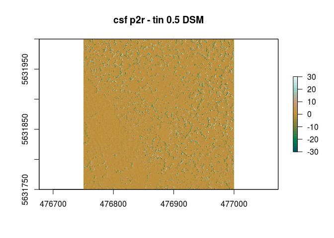
This looks a bit different if we look at the spatial differences.
# we need to resample the plus1 pixel
dsm_p2r_csf<-raster::resample(dsm_p2r_csf[[1]],dsm_pitfree_csf)
r<- dsm_pitfree_csf[[1]]- dsm_tin_csf[[1]]
r[r<minValue(r)]<-minValue(r)
raster::plot(dsm_pitfree_csf- dsm_p2r_csf ,col=pal(32),main="csf pitfree -p2r 0.5 DSM")
raster::plot(r ,col=pal(32),main="csf pitfree - tin 0.5 DSM")
raster::plot(dsm_p2r_csf- dsm_tin_csf ,col=pal(32),main="csf p2r - tin 0.5 DSM")
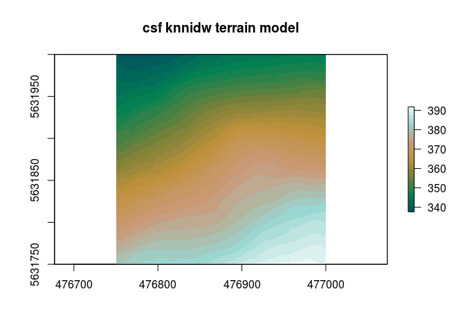
Same situation with the Digital Terrain Models. Here we are using to different approaches.
lidR::opt_output_files(mof_snip_ground_csf)<-paste0(path$data_lidar_level1_example,"{ID}_knn_csf")
dtm_knn_csf = lidR::grid_terrain(mof_snip_ground_csf, res=0.5,  algorithm = lidR::knnidw(k=50, p=3))
raster::plot(dtm_knn_csf,col=pal(32),main="csf knnidw terrain model")
lidR::opt_output_files(mof_snip_ground_csf)<-paste0(path$data_lidar_level1_example,"{ID}_gtin_csf")
dtm_tin_csf = lidR::grid_terrain(mof_snip_ground_csf, res=0.5,  algorithm = lidR::tin())
raster::plot(dtm_tin_csf,col=pal(32),main="csf knnidw terrain model")
If we check the difference of both models we see they are identical.
summary(dtm_tin_csf - dtm_knn_csf)## layer
## Min. 0
## 1st Qu. 0
## Median 0
## 3rd Qu. 0
## Max. 0
## NA's 0
The creation of a canopy Height model is a simple difference bettween DSM and DTM.
raster::plot(dsm_p2r_csf - dtm_knn_csf,col=pal(32), main="dsm_p2r_csf - dtm_knn_csf 0.5m CHM")
raster::plot(dsm_pitfree_csf - dtm_knn_csf, col=pal(32),main="dsm_pitfree_csf - dtm_knn_csf 0.5m CHM")
raster::plot(dsm_tin_csf - dtm_knn_csf, col=pal(32),main="dsm_tin_csf - dtm_knn_csf 0.5m CHM")
summary(dsm_p2r_csf - dtm_knn_csf)## layer
## Min. -0.1687012
## 1st Qu. 16.9708176
## Median 20.7978516
## 3rd Qu. 23.3927917
## Max. 32.4472961
## NA's 0.0000000
summary(dsm_pitfree_csf - dtm_knn_csf)## layer
## Min. -0.4230347
## 1st Qu. 16.9303665
## Median 20.7596283
## 3rd Qu. 23.3599625
## Max. 32.3883972
## NA's 0.0000000
summary(dsm_tin_csf - dtm_knn_csf)## layer
## Min. -0.4230347
## 1st Qu. 16.9303665
## Median 20.7596283
## 3rd Qu. 23.3599625
## Max. 32.3883972
## NA's 0.0000000
Basically therre are no huge differences in the results. Nevetheless this may change with poorer data or different parameters. You always have to try and to decide. Especially Martin Isenburgs blog posts from rapidlasso are always an very good first address. Even if LAStools are commercial Martin is sharing an incredible knowledge in dealing with LiDAR data. The R package lidR is an extremly powerful tool to deal with most of this issues from an open source point of view.