-
Notifications
You must be signed in to change notification settings - Fork 17
High resolution UAV digital terrain models generated RGB image data
Digital Terrain and Surface Models (DTM/DSMs) are probably the most used common data sets ever. High resolution DSM/DTM are nowadays usually derived from LiDAR data. However they have a poor repetition rate, the retrieval is expensive and not always and everywhere possible or available. Lowest budget ready to fly unmanned vehicles (rtf-UAVs) are very suitable to close this gap for a fast and reasonable retrieval of imagery data. Nevertheless due to the fact that optical imagery only can see surfaces and cameras can not take pictures from inside the forests and other more or less opaque structures. As a result the derived dense point clouds (DPCs) are more surface points clouds (SPCs).
The aim of this short tutorial is to show some possibilities to do so.
To derive Orthoimages or point clouds one can use between different tools the tutorial data is produced using Agisoft Photoscan which is a great tool for deriving point clouds and all kind of surface models. At the end of the Agisoft processing chain you will have an orthorectified image and a dense point cloud. We will use some UAV data from the Marburg Open Forest project.
First we have to set up the project. Because a bunch of software is needed we create a fix structure and link them against R.
devtools::install_github("gisma/uavRst", ref = "develop")
require(raster)
require(mapview)
require(link2GI)

# proj subfolders
projRootDir<-tempdir()


paths<-link2GI::initProj(projRootDir = projRootDir,
                         projFolders = c("data/","data/ref/","output/","run/","las/"),
                         global = TRUE,
                         path_prefix = "path_")

# get some colors
pal = mapview::mapviewPalette("mapviewTopoColors")

# get the data
# NOTE file size is about 80MB

utils::download.file(url="https://github.com/gisma/gismaData/raw/master/uavRst/data/477369_800_5631924_000_477469_800_5632024_000.las",
destfile=paste0(path_data,"lasdata.las"))

# make the folders and linkages
# NOTE this will take some time - especially running Windows
giLinks<-uavRst::linkAll() We take the original resolution without any filtering.
# calculate DSM uav point cloud
dsm1 <- uavRst::pc2D_dsm(laspcFile = paste0(path_data,"lasdata.las"),
                         gisdbasePath = projRootDir,
                         sampleMethod = "mean",
                         targetGridSize = 0.02,
                         giLinks = giLinks)
## :: create copy of the las file at the working directory...
## :: get extent of the point cloud
## :: link to GRASS
## :: sampling mean altitudes using : 0.02 meter grid size
## :: filling no data values if so
pal = mapviewPalette("mapviewTopoColors")
raster::plot(dsm1,col = pal(100), main ="0.02m  DSM")
We want 0.25 meter resolution without filtering.
dsm2 <- uavRst::pc2D_dsm(laspcFile = paste0(path_data,"lasdata.las"),
                         gisdbasePath = projRootDir,
                         sampleMethod = "mean",
                         targetGridSize = 0.25,
                         giLinks = giLinks)
## :: create copy of the las file at the working directory...
## :: get extent of the point cloud
## :: link to GRASS
## :: sampling mean altitudes using : 0.25 meter grid size
## :: filling no data values if so
pal = mapviewPalette("mapviewTopoColors")
raster::plot(dsm2,col = pal(100), main ="0.25m  DSM")
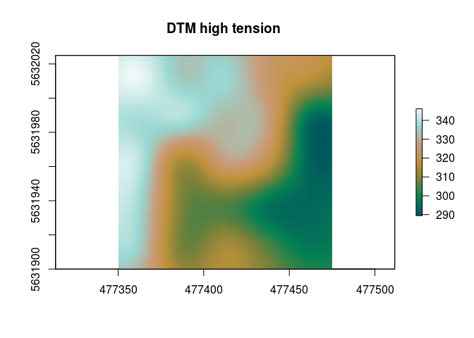
It is a bit tricky to get the right setting. There are a lot of problems to deal with. Basically spoken we need to mark all points that are lower in comparison to the direct neighborhoud. However this can be done by several algorithms and tools but all of them are optimized for LiDAR data sets. the example data is preclassified by Agisoft Photoscan but with a high bias. So the crucial parameters is a correct balance of thin_with_gridfor thinnig the point cloud data and level_max for the level of the multi-level spline interpolation.
dtm1 <- uavRst::pc2D_dtm_fw(laspcFile = paste0(path_data,"lasdata.las"),
                        gisdbasePath = tempdir(),
                        tension = 50 ,
                        targetGridSize = 1,
                        giLinks = giLinks)
## :: create copy of the las file at the working directory...
## :: get extent of the point cloud
## :: sampling minimum altitudes using : 25 meter grid size
## :: create DTM by interpolation to a raster size of: 1
raster::plot(dtm1,col = pal(100), main ="DTM high tension ")
We want to have a smooth result that keeps the terrain structures as much as possible, so we can change the filter and resolution options. Less Thinning and a higher filter.
dtm2 <- uavRst::pc2D_dtm_fw(laspcFile = paste0(path_data,"lasdata.las"),
                        gisdbasePath = tempdir(),
                        tension = 5 ,
                        targetGridSize = 1,
                        giLinks = giLinks)
## :: create copy of the las file at the working directory...
## :: get extent of the point cloud
## :: sampling minimum altitudes using : 25 meter grid size
## :: create DTM by interpolation to a raster size of: 1
raster::plot(dtm2,col = pal(100), main ="DTM low tension ") DTM third attempt ------------------
We use the multiscale auto adaption version of the pc2D_dtm Algorithm which tries to find an optimal balance between local detail and overall terrain structure.
dtm3 <- uavRst::pc2D_dtm(laspcFile = paste0(path_data,"lasdata.las"),
                        gisdbasePath = tempdir(),
                        targetGridSize = 1,
                        giLinks = giLinks)
## :: create copy of the las file at the working directory...
## :: create DTM by interpolation to a raster size of: 1
raster::plot(dtm3,col = pal(100), main ="DTM multiscale ")
Keeping in mind that we do not have any reliable knowledge of what is surface of the bare ground or buildings forest canopies or whatever, it will be an explorative and adaptive task to optimize the paramter settings for a reliable result.