-
Notifications
You must be signed in to change notification settings - Fork 3
Part 9: Dimensionality Reduction
The reason why we need it is covered in here.
Feature selection is used for filtering irrelevant or redudant features from the dataset.
Differences between selection and extraction is that feature selection keeps a subset of the original features while feature extraction creates brand new ones.
Feature selection can be unsupervised (e.g. Variance thresholds) or supervised (e.g. Genetic Algorithms).
Remove features whose values don't change much from observation to observation (e.g. their variance falls below a threshold) as these features provide little value.
For example, a public health dataset where 96% of were for 35y.o, then the "Age" and "Gender" features can be eliminated without a major loss in information.
- Strengths: Based on solid intuition and features that don't change much also don't add much information.
- Weaknesses: Might not be sufficient for dimensionality reduction. Requires setting a variance threshold which can be tricky.
Remove features that are highly correlated with others (e.g.. its values change very similarly to another's), as these features provide redundant information.
Calculate all pair-wise correlations, and remove the features if the correlation between a pair of features is above a given threshold.
For example, a real-estate dataset with "Floor Area (Sq. Ft.)" and "Floor Area (Sq. Meters)" as separate features can be safely removed.
- Strengths: Based on solid intuition, and some algorithms are not robust to correlated features hence removing boosts performance.
- Weaknesses: Requires setting a correlation threshold which can be tricky. Built-in feature selection such as PCA is a better alternative.

(Source: elitedatascience.com, n.d. - Good summary, open new tab to see it)
Search algorithms inspired by evolutionary biology and natural selection, combining mutation and cross-over to efficiently traverse large solution spaces.
The uses in ML is optimization and another is finding best weights for a Neural network, and another for supervised feature selection.
The "genes" represents individual features and "organism" represents a candidate set of features. Each organism in the "population" is graded on a fitness score such as model performance on a hold-out set.
The fittest "organisms" survive and reproduce, repeating until the "population" converges on a solution some generations later.
- Strengths: Efficiently select features from very high dimensional datasets where exhaustive search is unfeasible.
- Weaknesses: Adds higher level of complexity to implementation.
Feature extraction creates new and smaller set of features that stills captures most of the useful information.
Examples includes LDA and PCA.

(Source: Will, 2011)
It can be thought of as fitting a p-dimensional ellipsoid to the data, where each axis represents a principal component (e.g. PC1, PC2, ... - to dimension p).
If some axis of the ellipsoid is small, it indicates that the variance along that axis is also small.
In summary, to find the axes of the ellipsoid,
- Subtract the mean of each variable from the dataset to center the data around origin.
- Compute the covariance matrix of the data.
- Calculate the eigenvalues and corresponding eigenvectors of this covariance matrix.
- Normalize each of the orthogonal eigenvectors to turn them into unit vectors.
Unit eigenvectors can be interpreted as an axis of the ellipsoid fitted to the data. The proportion of the variance each eigenvector represents can be calculated by dividing the eigenvalue corresponding to that eigvenvector by the sum of all eigenvalues.
Using this standard dataset,

(Source: The Nobles, 2020)
Standardize the dataset by calculating the mean () and standard deviation (
) for each feature (axis).
This should lead us to the following

(Source: The Nobles, 2020)
Then applying the formula for each feature in the dataset transforms into,

(Source: The Nobles, 2020)
2. Calculate the Covariance matrix
Using the formula below (where represents the total number of data points, and
the dimensions or number of features),
This should lead us to the following,


(Source: The Nobles, 2020)

(Source: The Nobles, 2020)
To find the eigenvalues, solve the following equations,
This should give us the following,
λ = 2.51579324, 1.0652885, 0.39388704, 0.02503121

(Source: The Nobles, 2020)
Then, to find the eigenvectors, solve the following equations for each eigenvalue where,
This should give us each eigenvectors for each features (or eigenvalues), which is,

(Source: The Nobles, 2020)
Sort the eigenvalues by descending order and select the eigenvectors based on the top eigenvalues corresponding vectors.
This should give us the vectors for λ = 2.51579324, 1.0652885,

(Source: The Nobles, 2020)
Apply the following formula,
(Feature matrix) * (top eigenvectors) = (transformed data)
And this should derive us the following,

(Source: The Nobles, 2020)
Using SVD for Linear PCA
Imagine a matrix such as,
To obtain the SVD parameters,
For matrix , find the following,
Then calculate the eigenvectors and eigenvalues, where each eigenvectors is normalized,
For matrix , find the following,
Then calculate the eigenvectors and eigenvalues, where each eigenvectors is normalized,
Then it should be use to form matrices such that,
The co-variance matrix can be calculated as such,
Where,

(Source: Sebastian Raschka, 2015
Steps to achieve such,
- Choose a kernel function
.
- Compute Gram/Kernel matrix with each
.
- Center the kernel matrix
- Find eigenvectors
.
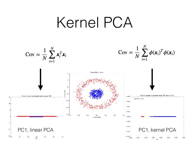
Kernel functions can be,

(Source: Gopi Sumanth, 2019)
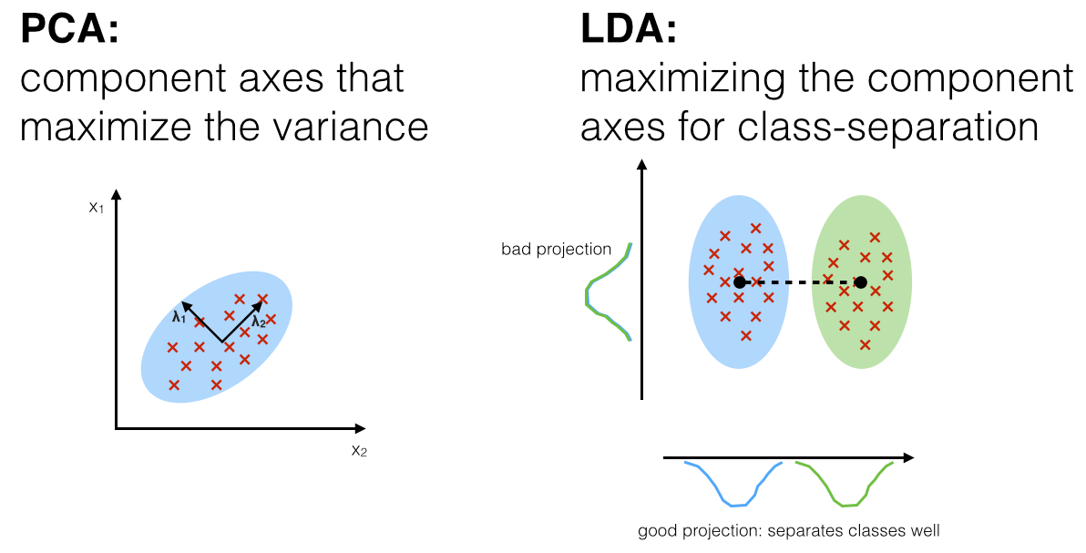
LDA, similar to PCA is a method of dimensionality reduction. However, they are different in approaches as PCA chooses new axes for dimensions such that variance of the data is preserved, but LDA chooses new axes such that the separability between classes is optimized.

(Source: Andre Ye, 2020)
This calculates the distances between classes and allows for the algorithm to put a quantitative measure on the difficulty of the problem, as closer means it is a harder problem.

(Source: Andre Ye, 2020)
This is the distance between the mean and the sample of every class, and another factor in the difficulty of separation, where the higher variance within a class makes clean separation more difficult.
This is known as the Fisher’s Criterion, where it is the ratio of the between-class scatter to the within-class scatter (read more here).
By maximizing this criterion, this maximizes the between-class variance ("separability") and minimizes the within-class variance.
Then, the optimal discriminant projection axis can be obtained.
This can be computed using SVD, eigenvalues or least-squares method.
Consider a very noisy two-dimensional scatterplot with two classes, projected by LDA into one dimension,

(Source: Andre Ye, 2020)
The separation is much more clear and distinct.
Or consider the MNIST dataset, whose 784 dimensions correspond each to one pixel in a (28 × 28) image of handwritten digits each from 0-9,

(Source: Andre Ye, 2020)
See that it is pretty impressive that LDA still manages to plot out differences at such a low dimensionality, despite the amount of information expressed in 784 dimensions.