Neural spectrum encoder and decoder
- Paper I (SDSS): https://arxiv.org/abs/2211.07890
- Paper II (SDSS): https://arxiv.org/abs/2302.02496
- Paper III (DESI EDR): https://arxiv.org/abs/2307.07664
From a data-driven side, galaxy spectra have two fundamental degrees of freedom: their instrinsic spectral properties (or type, if you believe in such a thing) and their redshift. The latter makes them awkward to ingest because it stretches everything, which means spectral features don't appear at the same places. This is why most analyses of the intrinsic properties are done by transforming the observed spectrum to restframe.
We decided to do the opposite. We build a custom architecture, which describes the restframe spectrum by an autoencoder and transforms the restframe model to the observed redshift. While we're at it we also match the spectral resolution and line spread function of the instrument:

Doing so clearly separates the responsibilities in the architecture. Spender establishes a restframe that has higher resolution and larger wavelength range than the spectra from which it is trained. The model can be trained from spectra at different redshifts or even from different instruments without the need to standardize the observations. Spender also has an explicit, differentiable redshift dependence, which can be coupled with a redshift estimator for a fully data-driven spectrum analysis pipeline.
The easiest way is pip install spender. When installing from the code repo, run pip install -e ..
For the time being, you will have to install one dependency manually: torchinterp1d is available here.
We make the best-fitting models discussed in the paper available through the Astro Data Lab Hub. Here's a workflow:
import torch.hub
github = "pmelchior/spender"

# get the spender code and show list of pretrained models
torch.hub.list(github)

# print out details for SDSS model from paper II
print(torch.hub.help(github, 'sdss_II'))

# load instrument and spectrum model from the hub
sdss, model = torch.hub.load(github, 'sdss_II')

# if your machine does not have GPUs, specify the device
from accelerate import Accelerator
accelerator = Accelerator(mixed_precision='fp16')
sdss, model = torch.hub.load(github, 'sdss_II', map_location=accelerator.device)catalog of latent-space probabilities for
- SDSS-I main galaxy sample; see Liang et al. (2023a) for details
- DESI EDR BGS sample; see Liang et al. (2023b) for details
Documentation and tutorials are forthcoming. In the meantime, check out train/diagnostics.ipynb for a worked through example that generates the figures from the paper.
In short, you can run spender like this:
import torch
from accelerate import Accelerator

# hardware optimization
accelerator = Accelerator(mixed_precision='fp16')

# get code, instrument, and pretrained spectrum model from the hub
github = "pmelchior/spender"
sdss, model = torch.hub.load(github, 'sdss_II',  map_location=accelerator.device)

# get some SDSS spectra from the ids, store locally in data_path
from spender.data.sdss import SDSS
data_path = "./DATA"
ids = ((412, 52254, 308), (412, 52250, 129))
spec, w, z, norm, zerr = SDSS.make_batch(data_path, ids)

# run spender end-to-end
with torch.no_grad():
  spec_reco = model(spec, instrument=sdss, z=z)

# for more fine-grained control, run spender's internal _forward method
# which return the latents s, the model for the restframe, and the observed spectrum
with torch.no_grad():
  s, spec_rest, spec_reco = model._forward(spec, instrument=sdss, z=z)

# only encode into latents
with torch.no_grad():
  s = model.encode(spec)
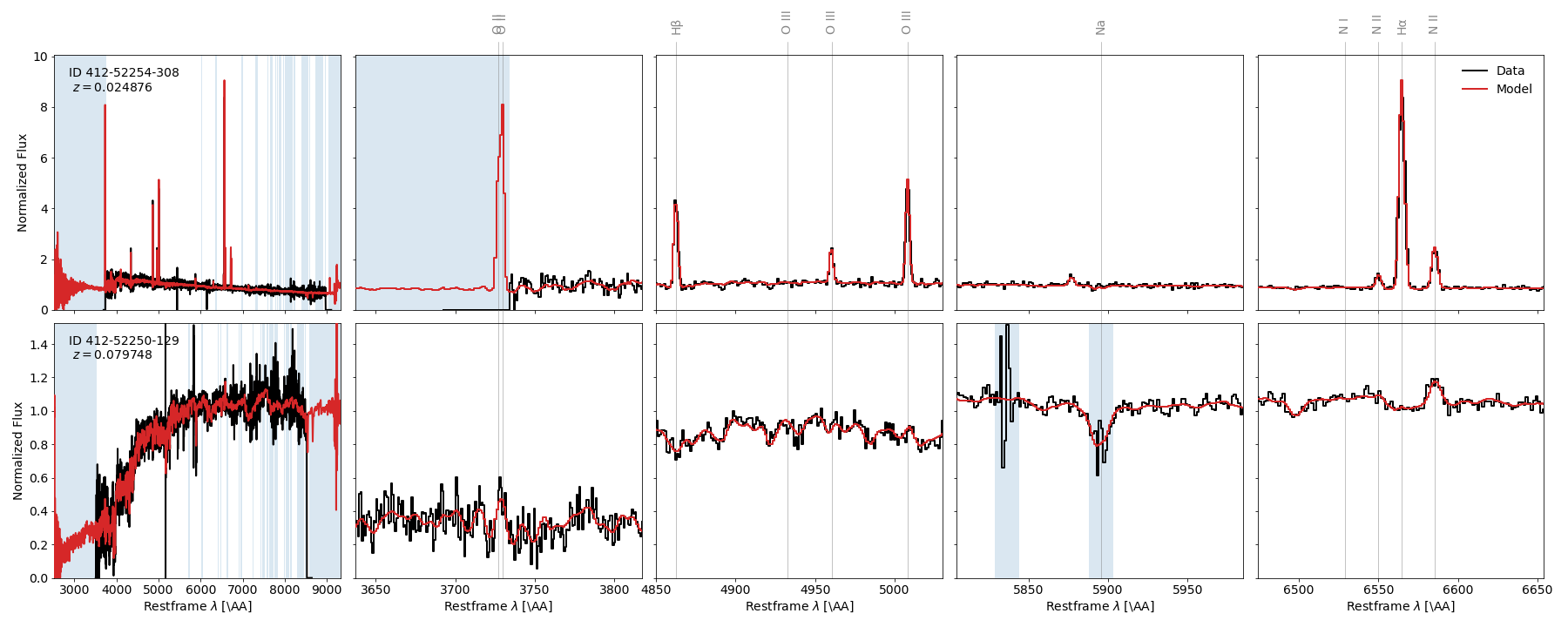
Plotting the results of the above nicely shows what spender can do:
Noteworthy aspects: The restframe model has an extended wavelength range, e.g. predicting the [O II] doublet that was not observed in the first example, and being unaffected by glitches like the skyline residuals at about 5840 A in the second example.
