A.01 Vectors
A coordinate system, also called frame, is a fundamental concept in mathematics and geometry. It provides a way to uniquely determine a position in space by using one or more numbers called coordinates.
To define a coordinate system, we need three key components: an origin, a unit of measurement, and a positive direction. The origin is a reference point from which all positions are measured. The unit of measurement determines the scale or size of each coordinate value. The positive direction indicates which way the coordinates increase from the origin.
By using a coordinate system, we can bridge the gap between geometry and numerical problems. Geometrical problems involving positions, distances, angles, and shapes can be translated into numerical problems by assigning coordinates to the geometric elements. Similarly, numerical problems can be visualized and understood geometrically by mapping the numbers that represent points and other geometric entities onto a coordinate system.
A 1D coordinate system is a simplified version of a coordinate system that operates along a single dimension, typically represented by a straight line or a curve. In a 1D coordinate system, we typically define an origin point as a reference point on the line. This origin point serves as the starting point from which positions are measured. We also must establish a unit of measurement, that determines the scale or increment used to quantify distances or positions along the line, and a positive direction, that indicates the direction in which the values increase from the origin. In this type of coordinate system, we can determine a position
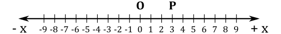
For example,
In the plane, two perpendicular lines (also called axes) are chosen, and the coordinates
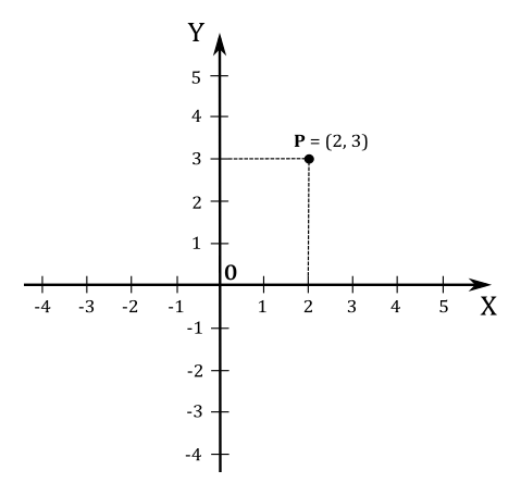
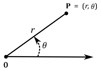
For example, the point
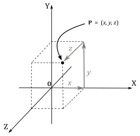
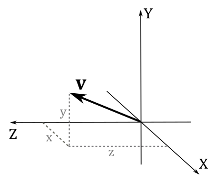
In three dimensions, three mutually orthogonal axes are chosen and the coordinates
You can also see the coordinates
Depending on the direction and order of the axes, a three-dimensional system may be a right-handed or a left-handed system.
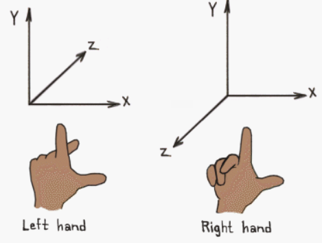
Typically, the y-axis points up, the x-axis points right while the z-axis points forward (note that forward aims at different directions depending on whether a right-handed or left-handed coordinate system is being used). That’s not a strict rule, though. Sometimes, you can have the z-axis points up, and in that case the y-axis points forward. You can always switch from a y-up to a z-up configuration with a simple transformation, but there's no point in providing further details here as we will use z-up or y-up configurations consistently during the rendering process (further details will be provided as needed). Apparently, it seems that right-handed coordinate systems are commonly used by Vulkan programmers, so we will follow this convention in this tutorial series as well. However, again, it is not a strict rule and left-handed coordinate systems can also be used.
In a two-dimensional plane, we can define a coordinate system known as polar coordinate system. This system is based on a reference point called origin or pole and a ray extending from the origin called polar axis. A point
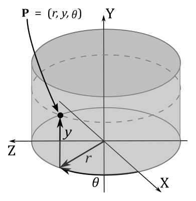
In three dimensions, we extend the polar coordinate system with an additional y-coordinate to specify the height of a point. That way, we can locate all the points of a cylinder. That’s why we call
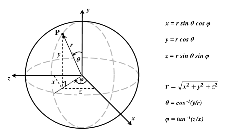
Spherical coordinates use a similar approach by adding another angle
In homogeneous coordinates, a point in the plane can be represented by a triple
Vectors are mathematical objects that represent quantities with both magnitude and direction. They are used in many fields, including physics and computer graphics. For example, vectors can be used to specify the position and displacement of objects in space, as well as their speed. They can also describe the direction and intensity of forces acting on objects or light rays emitted by a light source, as well as the surface normal.
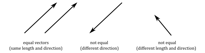
Geometrically, a vector can be visualized as an arrow. The length of the arrow represents the magnitude or size of the vector, while the direction in which the arrow points indicates the direction of the vector.
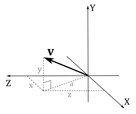
When working with vectors on a computer, the geometric definition provided above is not as important, although. Fortunately, we can express vectors numerically using tuples, which are finite sequences of numbers. To establish this numerical representation, we need to bind vectors to the origin of a Cartesian coordinate system. In other words, we translate a vector while maintaining its magnitude and direction until its starting point aligns with the origin.
At that point, we can use the coordinates
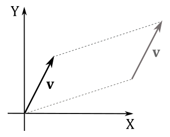
When only magnitude and direction of a vector matter, then the point of application is of no importance, and the vector is called free vector. On the other hand, a vector bound to the origin of a system is called bound vector. The numerical representation of a bound vector is only valid in the system where it is bound. If the same free vector is bound to different systems, its numerical representation will change accordingly.
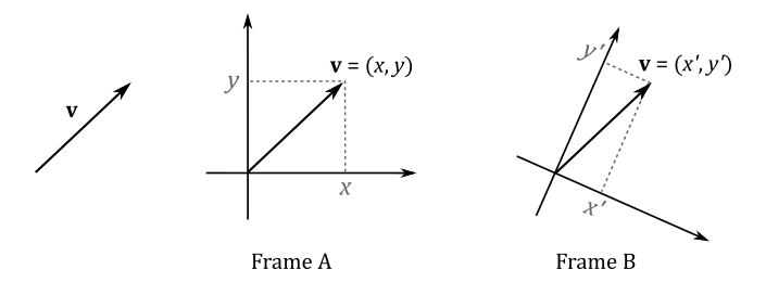
This is an important point to remember: if you define a vector numerically, its coordinates are relative to a specific frame of reference. Therefore, we can conclude that two vectors
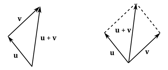
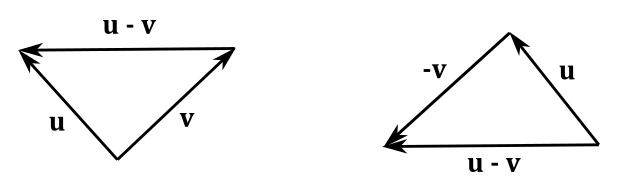
Numerically, the sum of two vectors
The addition may be represented geometrically by placing the tail of the arrow representing
The difference between two vectors
Geometrically, the vector subtraction can be defined by bounding
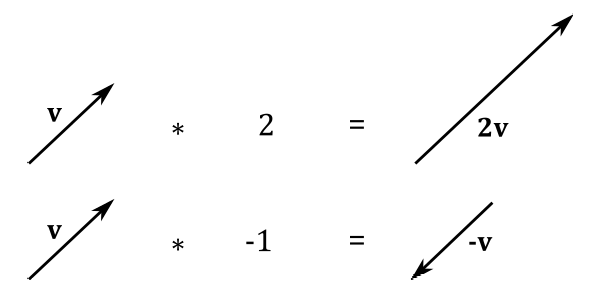
We can multiply a vector
Geometrically, this is equivalent to scaling a vector, which is why real numbers are often called scalars. If
Here are some of the properties of vector addition and scalar multiplication:
| Commutative (vector) | |
| Associative (vector) | |
| Additive Identity |
|
| Distributive (vector) | |
| Distributive (scalar) | |
| Associative (scalar) | |
| Multiplicative Identity |
|
Now we can define the length of a vector
We have that
Sometimes, only the direction of a vector is relevant. In such cases, we can normalize the vector to ensure its length becomes 1. Usually, the symbol
We can verify that
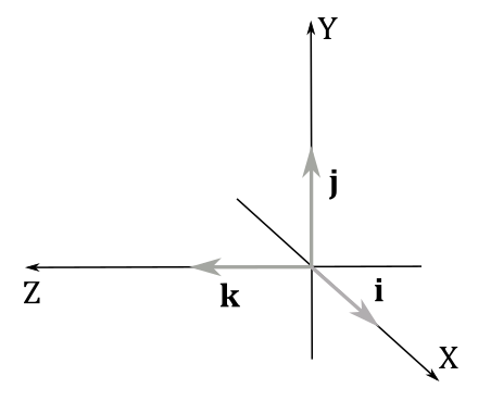
Three significant unit vectors are:
The dot product is a form of vector multiplicatio that results in a scalar value. It is also known as the scalar product for this reason. The dot product of two vector
So, the dot product of two vectors is obtained by summing the products of their corresponding components. Below are some of the properties of the dot product:
| Commutative | |
| Distributive | |
| Square of a vector length |
The associative property doesn’t apply because
From the law of cosines
Indeed, if we set
From equation
- If
$(\mathbf{u}\cdot\mathbf{v}) = 0$ then the angle$\theta$ between$\mathbf{u}$ and$\mathbf{v}$ is$90°$ (that is, they are orthogonal:$\mathbf{u}\ \bot\ \mathbf{v}$ ) - If
$(\mathbf{u}\cdot\mathbf{v}) > 0$ then the angle$\theta$ between$\mathbf{u}$ and$\mathbf{v}$ is less than$90°$ - If
$(\mathbf{u}\cdot\mathbf{v}) < 0$ then the angle$\theta$ between$\mathbf{u}$ and$\mathbf{v}$ is greater than$90°$
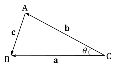
To conclude this section, we will prove the law of cosines
Let
$\mathbf{a}$ be the vector from$C$ to$B$ ,$\mathbf{b}$ the vector from$C$ to$A$ , and$\mathbf{c}$ the vector from$A$ to$B$ .
We have that
$\mathbf{c}=\mathbf{a}-\mathbf{b}\quad$ (subtration of two vectors)Squaring both sides and simplifying
$|\mathbf{c}|^2=|\mathbf{a}-\mathbf{b}|^2$
$|\mathbf{c}|^2=(\mathbf{a}-\mathbf{b})\cdot (\mathbf{a}-\mathbf{b})\quad\quad\quad\quad\quad\quad\quad\quad$ (square of a vector length)
$|\mathbf{c}|^2=|\mathbf{a}|^2+|\mathbf{b}|^2-2\ \mathbf{a}\cdot\mathbf{b}\quad\quad\quad\quad\quad\quad\quad$ (distributive law of the dot product)
$|\mathbf{c}|^2=|\mathbf{a}|^2+|\mathbf{b}|^2-2|\mathbf{a}||\mathbf{b}| \cos{\theta}\quad\quad\quad\quad$ (equation (1))
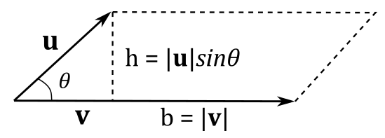
The orthogonal projection of a vector
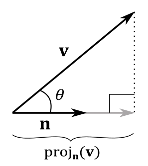
From trigonometry, we know that in a right triangle, the cosine of an angle is equal to the ratio of the length of the adjacent side to the length of the hypotenuse. Therefore, we can calculate the length of the adjacent side by multiplying the length of the hypotenuse by the cosine of the angle between the adjacent side and the hypotenuse. Considering the illustration above, we have that
with
Thanks to the concept of orthogonal projection, we can express any bound vector
Indeed, we have
Also, note that
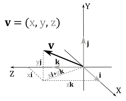
You can also see it as a sum of scaled vectors: we scale
Remember that you can also see it as a sequence of three translations: starting from the origin of the frame, we move
As stated earlier, the components of a bound vector represent the coordinates of its arrowhead within the frame. This allows us to uniquely identify all points within a frame using vectors. However, we still need a way to distinguish between vectors and points, as they are not interchangeable. For vectors, only their direction and magnitude matter, making the point of application irrelevant. On the other hand, points uniquely represent a location and only make sense when bound to the origin of a frame. Subtracting points yields a vector that specifies the movement from one point to another, while adding a point and a vector gives a vector that specifies how to move a point to a different location. However, unlike vectors, adding two points does not have a meaningful interpretation - geometrically it's the diagonal of a parallelogram, but this interpretation is not particularly useful or relevant when working with points.
In summary, consider vectors as free vectors and points as bound vectors. When working with a generic vector
A computer cannot exactly represent all the elements in the infinite set of real numbers because it uses a finite number of bits to store values in memory. This means we have to settle for a good approximation. The downside is that, if you need to perform many calculations with approximate values, the outcome could differ significantly from the exact result. For example, a set of vectors
Suppose we have an initial set of vectors
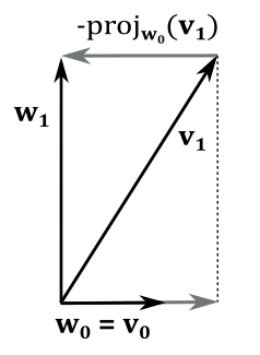
So, we have that
where
To prove that
In the 3D case, we introduce a third vector
To calculate
Consider the following illustration. If we subtract
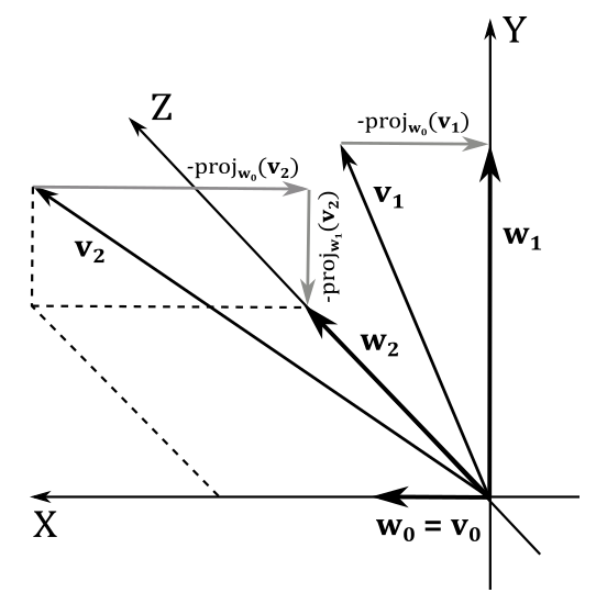
The final step in the process of orthogonalization is to normalize the vectors
This type of multiplication is also called vector product as the result is a vector (unlike the dot product which evaluates to a scalar). The cross product is defined as
A way to remember this formula is to notice that the first component of the vector
We can also use matrices to calculate the cross product. For example, the cross product
$\mathbf{u}\times\mathbf{v}$ is equal to the determinant of the$3\times 3$ matrix with$\mathbf{i}$ ,$\mathbf{j}$ and$\mathbf{k}$ as elements of the first row, and the components of the two vectors$\mathbf{u}$ and$\mathbf{v}$ as elements of the other two rows.
$\mathbf{w}=\mathbf{u}\times\mathbf{v}=\left\lvert\matrix{\mathbf{i} & \mathbf{j} & \mathbf{k} \cr u_x & u_y & u_z \cr v_x & v_y & v_z}\right\rvert=$
$(u_y v_z-u_z v_y)\mathbf{i}-(u_x v_z-u_z v_x)\mathbf{j}+(u_x v_y-u_y v_x)\mathbf{k}=$
$(u_y v_z-u_z v_y,\ u_z v_x-u_x v_z,\ u_x v_y-u_y v_x)$
Also, the cross product can be computed multiplying a matrix by a column.
$\mathbf{w}=\mathbf{u}\times\mathbf{v}=\left\lbrack\matrix{0&-u_z&u_y \cr u_z&0&-u_x \cr -u_y&u_x&0}\right\rbrack\left\lbrack\matrix{v_x\cr v_y\cr v_z}\right\rbrack=$
$(u_yv_z-u_zv_y,\ u_zv_x-u_xv_z,\ u_xv_y-u_yv_x)$
We will cover matrices in the next appendix, where we will show that the determinant of a matrix is related to the concept of hypervolume (that is, length in 1D, area in 2D, and volume in 3D). However, in this section we can use the information provided in the box above to find something interesting. We know that two vectors always lie in a plane, and that to calculate the area of a parallelogram we multiply its base times the height. Then, we are supposed to find a similar formula for the cross product because, to compute it, we can use the determinant of a matrix, which is related to the concept of hypervolume. Indeed, we can also write the cross product as follows
with
We know that
since
As just stated above, the vector
In left-handed systems, the correct side is the one that makes
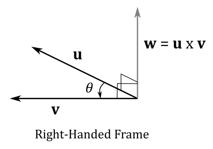
The commutative property doesn’t apply
And we also have that
A way to remember the above equivalences is to consider the unit vectors
The scalar triple product is nothing really new, as it simply combines the dot product and the cross product. It is defined as:
where
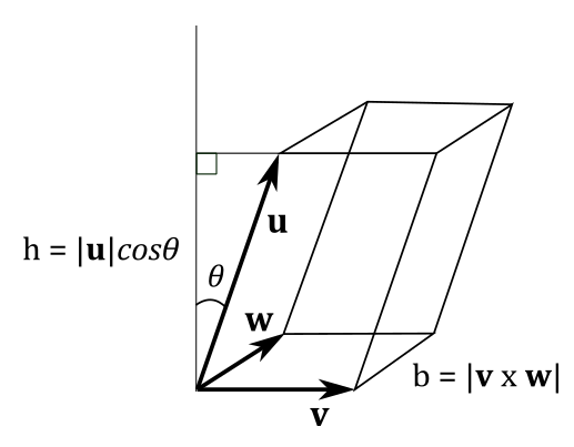
As you know, the length of the cross product is the area of a parallelogram. Also, the volume of a parallelepiped is
with
From equation
which is the scalar triple product. If you expand it you have
which is exactly the determinant of the
We conclude this section pointing out that a vector triple product
$\mathbf{a}\times (\mathbf{b}\times\mathbf{c})=(a_x, a_y, a_z)\times [(b_x, b_y, b_z)\times (c_x, c_y, c_z)]=$
$(a_x,, a_y,, a_z)\times (b_yc_z-b_zc_y,; b_zc_x-b_xc_z,; b_xc_y-b_yc_x)=$
$\big({\color{#FF6666}{a_y (b_xc_y-b_yc_x)-a_z (b_zc_x-b_xc_z)}},\ {\color{#44FF66}{a_z (b_yc_z-b_zc_y)-a_x\ (b_xc_y-b_yc_x)}},\ {\color{#44AAFF}{a_x (b_zc_x-b_xc_z)-a_y(b_yc_z-b_zc_y)}}\big)$
Below we can see that the first component of
$\mathbf{b}(\mathbf{a}\cdot\mathbf{c})-\mathbf{c}(\mathbf{a}\cdot\mathbf{b})$ is equivalent to the first component of$\mathbf{a}\times(\mathbf{b}\times\mathbf{c})$
$(\mathbf{b}(\mathbf{a}\cdot\mathbf{c})-\mathbf{c}(\mathbf{a}\cdot\mathbf{b}))_x = b_x (a_xc_x+a_yc_y+a_zc_z)-c_x (a_xb_x+a_yb_y+a_zb_z)=$
$a_xb_xc_x+a_yb_xc_y+a_zb_xc_z-a_xb_xc_x-a_yb_yc_x-a_zb_zc_x=$
${\color{#FF6666}{a_y (b_xc_y-b_yc_x)-a_z (b_zc_x-b_xc_z)}}$
The same applies to the other two components.
Vectors play a crucial role in computer graphics, making them a fundamental tool to use in Vulkan as well. They are widely used in both C++ (within the application code) and in GLSL (within shader code).
In GLSL, vectors of two, three and four floating-point components are represented by the built-in types vec2, vec3 and vec4, respectively. For vectors of signed integers, we use ivec2, ivec3 and ivec4 - the unsigned version can be specified by replacing the prefix i with u.
The components of a vector can be accessed using array subscripting syntax to provide numeric indexing. Alternatively, one of the following naming sets can be used:
The position set:
The color set:
The texel set:
Specifying one or more vector components is called swizzling. For example:
ivec2 a = ivec2(1, 2);            // init using vector constructor
uvec3 b = { 1, 2, 3 };            // init using an initializer-list
uvec4 c = uvec4(b, 4);            // init using the component of another vector
vec4 d = vec4(c);                 // makes a vec4 with component-wise conversion (uint to float)

vec4 e = { 1.0, 2.0, 3.0, 0.0 };  // 1.0 means 1.0f (f suffix is implicit for floats)
float f0 = e.x;                   // f0 = 1.0f
float f1 = e.g;                   // f1 = 2.0f
float f2 = e[2];                  // f2 = 3.0f
e.a = 4.0f;                       // e = (1.0f, 2.0f, 3.0f, 4.0f)

vec4 f = { 1.0f, 2.0f, 3.0f, 4.0f };
vec3 g = f.xyz;                      // g = (1.0f, 2.0f, 3.0f)
vec2 h = f.rb;                       // h = (1.0f, 3.0f)
vec4 m = f.zzxy;                     // m = (3.0f, 3.0f, 1.0f, 2.0f)
m.wxyz = m;                          // m = (3.0f, 1.0f, 2.0f, 3.0f)
m.yw = g.zz;                         // m = (3.0f, 3.0f, 2.0f, 3.0f)

vec4 w = vec4(g, 5.0);               // w = (1.0f, 2.0f, 3.0f, 5.0f)
Using vectors in C++ is not as straightforward as in GLSL because there are no built-in types available. Indeed, while the header files provided by the Khronos Group include the graphical functionalities described in the Vulkan specification, they do not include the implementation of mathematical entities such as vectors. Therefore, we have to make a choice between implementing a mathematical library from scratch or using an existing and well-established one. Implementing such a library correctly is not a straightforward task, so we will rely on a proven library like GLM (OpenGL Mathematics), which is a header only C++ mathematics library for graphics software based on the OpenGL Shading Language (GLSL) specifications. However, as stated at the beginning of this tutorial series, I will not assume that the reader has any previous knowledge of computer graphics. Therefore, we will analyze the code of the structures and methods implemented in GLM to explain their theoretical foundations.
GLM provides the following types, which allow us to use integer or floating-point vectors.
typedef vec<1, float, defaultp>  vec1;
typedef vec<2, float, defaultp>  vec2;
typedef vec<3, float, defaultp>  vec3;
typedef vec<4, float, defaultp>  vec4;

typedef vec<1, int, defaultp>  ivec1;
typedef vec<2, int, defaultp>  ivec2;
typedef vec<3, int, defaultp>  ivec3;
typedef vec<4, int, defaultp>  ivec4;

typedef vec<1, uint, defaultp>	uvec1;
typedef vec<2, uint, defaultp>	uvec2;
typedef vec<3, uint, defaultp>	uvec3;
typedef vec<4, uint, defaultp>	uvec4;

// Similar structures are provided for vectors of one, two and three components
template<typename T, qualifier Q>
struct vec<4, T, Q>
{

    // ...


    // -- Data --

    union { T x, r, s; };
    union { T y, g, t; };
    union { T z, b, p; };
    union { T w, a, q; };

    // ...

}
Refer to the complete source code to see how conversions and constructors are implemented to mimic the GLSL behaviour. This approach will allow you to understand the practical implementation details without necessarily consulting the GLSL specification directly. For example, the following explicit conversion means that we can construct a vec4 from four components of different types, both in C++ and GLSL.
GLM
/// Explicit conversions (From section 5.4.1 Conversion and scalar constructors of GLSL 1.30.08 specification)
template<typename X, typename Y, typename Z, typename W>
GLM_FUNC_DECL GLM_CONSTEXPR vec(X _x, Y _y, Z _z, W _w);


template<typename T, qualifier Q>
template<typename X, typename Y, typename Z, typename W>
GLM_FUNC_QUALIFIER GLM_CONSTEXPR vec<4, T, Q>::vec(X _x, Y _y, Z _z, W _w)
    : x(static_cast<T>(_x))
    , y(static_cast<T>(_y))
    , z(static_cast<T>(_z))
    , w(static_cast<T>(_w))
{}
C++
// vec4 built from a signed int, a float, a double and a unsigned int; no suffix defined for doubles in C++
glm::vec4 a(-1, 2.0f, 3.0, 4u); // a = (1.0f, 2.0f, 3.0f, 4.0f)
GLSL
// vec4 built from a signed int, a float, a double and a unsigned int
vec4 a = vec4(-1, 2.0, 3.0lf, 4u); // doubles in GLSL need lf suffix (f for floats is implicit)
Obviously, all the basic vector operations discussed in this tutorial (sum, difference and various types of multiplication) are both defined in GLSL and implemented GLM, along with other geometric functions that can be performed on vectors such as normalization, length\magnitude calculation, reflection and many more. For example, the sum of two vec3 in GLM is defined exactly as per the definition (sum of the corresponding components).
template<typename U>
GLM_FUNC_DECL GLM_CONSTEXPR vec<3, T, Q> & operator+=(vec<3, U, Q> const& v);

//
template<typename T, qualifier Q>
template<typename U>
GLM_FUNC_QUALIFIER GLM_CONSTEXPR vec<3, T, Q> & vec<3, T, Q>::operator+=(vec<3, U, Q> const& v)
{
    this->x += static_cast<T>(v.x);
    this->y += static_cast<T>(v.y);
    this->z += static_cast<T>(v.z);
    return *this;
}
Similarly, you can verify that the normalization and the length of a vector
norm(v) = v * inversesqrt(dot(v, v));
length(v) = sqrt(dot(v, v));
Refer to the GLM code to verify that they are actually implemented this way.
In a later appendix, we will discuss other geometric functions that operate on vectors, such as reflection and projection.
Source code: LearnVulkan
[1] Practical Linear Algebra: A Geometry Toolbox (Farin, Hansford)
If you found the content of this tutorial somewhat useful or interesting, please consider supporting this project by clicking on the Sponsor button. Whether a small tip, a one time donation, or a recurring payment, it's all welcome! Thank you!